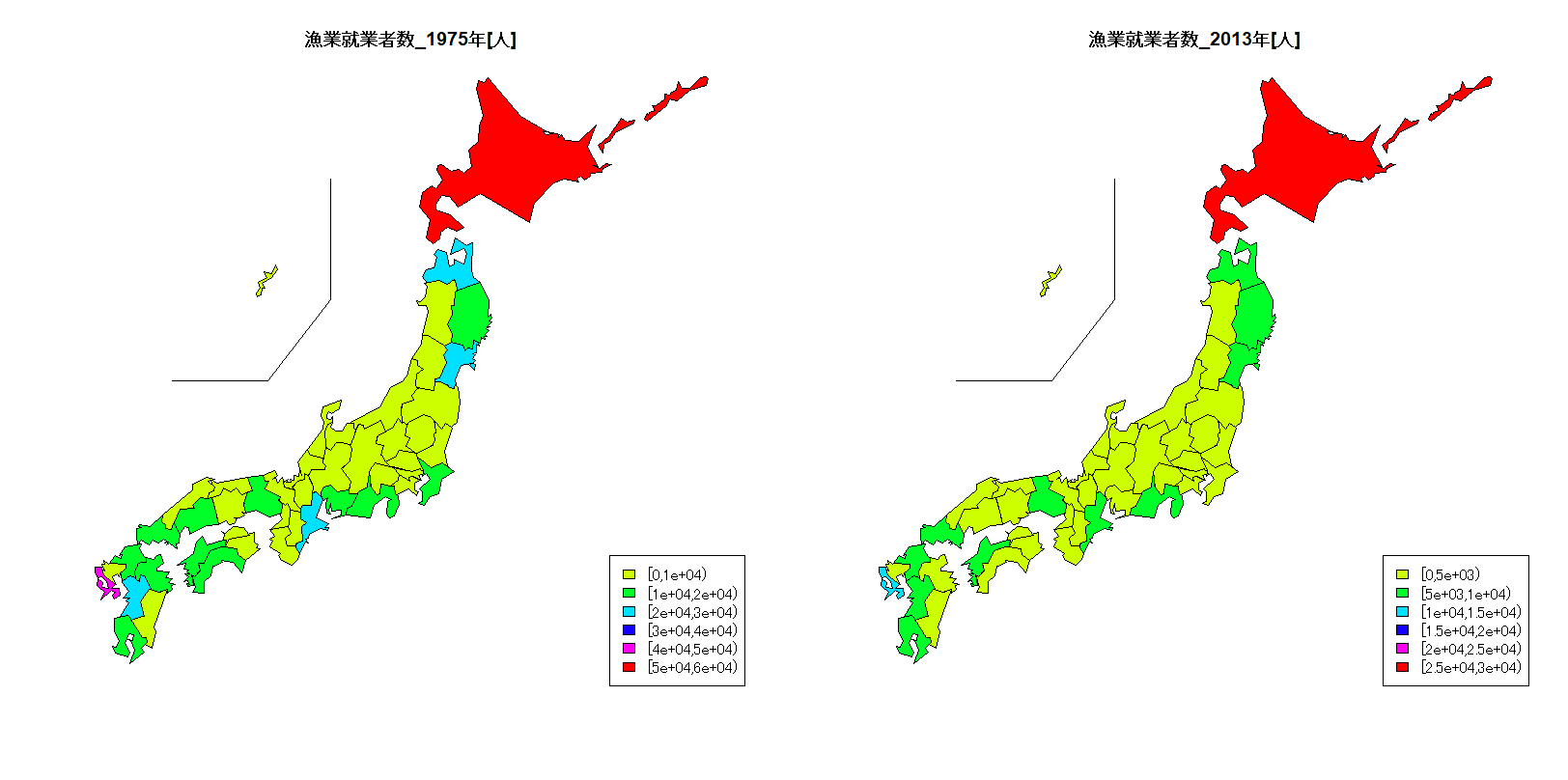
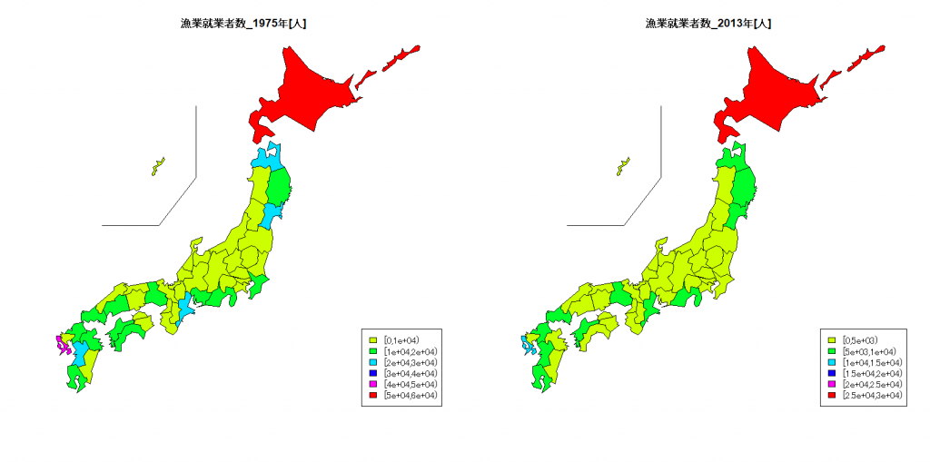
総務省統計局が発表している「都道府県・市区町村のすがた(社会・人口統計体系)」から、都道府県別の漁業就業者数[人]を1975年と2013年で比べてみます。
| 都道府県 |
漁業就業者数_1975 |
漁業就業者数_2013 |
| 北海道 |
50790 |
29652 |
| 青森 |
23310 |
9879 |
| 岩手 |
18900 |
6289 |
| 宮城 |
29150 |
6516 |
| 秋田 |
4750 |
1011 |
| 山形 |
2100 |
474 |
| 福島 |
4280 |
343 |
| 茨城 |
3280 |
1435 |
| 栃木 |
0 |
0 |
| 群馬 |
0 |
0 |
| 埼玉 |
0 |
0 |
| 千葉 |
16660 |
4734 |
| 東京 |
1890 |
972 |
| 神奈川 |
5290 |
2273 |
| 新潟 |
6380 |
2579 |
| 富山 |
3500 |
1428 |
| 石川 |
7570 |
3296 |
| 福井 |
3560 |
1735 |
| 山梨 |
0 |
0 |
| 長野 |
0 |
0 |
| 岐阜 |
0 |
0 |
| 静岡 |
13760 |
5750 |
| 愛知 |
12220 |
4319 |
| 三重 |
26010 |
7791 |
|
| 都道府県 |
漁業就業者数_1975 |
漁業就業者数_2013 |
| 滋賀 |
0 |
0 |
| 京都 |
2330 |
1421 |
| 大阪 |
1380 |
1036 |
| 兵庫 |
12220 |
5334 |
| 奈良 |
0 |
0 |
| 和歌山 |
8150 |
2907 |
| 鳥取 |
3010 |
1320 |
| 島根 |
9400 |
3032 |
| 岡山 |
4190 |
1658 |
| 広島 |
13790 |
4003 |
| 山口 |
17490 |
5106 |
| 徳島 |
6160 |
2512 |
| 香川 |
6590 |
2484 |
| 愛媛 |
19200 |
7416 |
| 高知 |
11910 |
3970 |
| 福岡 |
14400 |
5140 |
| 佐賀 |
9480 |
4260 |
| 長崎 |
41680 |
14310 |
| 熊本 |
22700 |
6882 |
| 大分 |
12620 |
4110 |
| 宮崎 |
5640 |
2677 |
| 鹿児島 |
16010 |
7200 |
| 沖縄 |
5610 |
3731 |
|
|
library(leaflet)
library(knitr)
library(kableExtra)
library(dplyr)
library(tidyr)
library(stringr)

dat <- read.csv("http://www.dinov.tokyo/Data/JP_Pref/Pref_data.csv", header = TRUE, fileEncoding="UTF-8")
col_start <- 0.2
col_end <- 0.0

table_df<-data.frame(都道府県=dat$都道府県, 漁業就業者数_1975=dat$漁業就業者数_1975, 漁業就業者数_2013=dat$漁業就業者数_2013)

datc_k <- cut(dat$漁業就業者数_1975, hist(dat$漁業就業者数_1975, plot=FALSE)$breaks, right=FALSE)
datc_kcol <- rainbow(length(levels(datc_k)), start = col_start, end=col_end)[as.integer(datc_k)]
datc_m <- cut(dat$漁業就業者数_2013, hist(dat$漁業就業者数_2013, plot=FALSE)$breaks, right=FALSE)
datc_mcol <- rainbow(length(levels(datc_m)), start = col_start, end=col_end)[as.integer(datc_m)]
windowsFonts(JP4=windowsFont("Biz Gothic"))
windows(width=1600, height=800)
par(family="JP4")
layout(matrix(1:2, 1, 2))

library(NipponMap)
JapanPrefMap(datc_kcol, main="漁業就業者数_1975年[人]")
legend("bottomright", fill=rainbow(length(levels(datc_k)), start = col_start, end=col_end), legend=names(table(datc_k)))
JapanPrefMap(datc_mcol, main="漁業就業者数_2013年[人]")
legend("bottomright", fill=rainbow(length(levels(datc_m)), start = col_start, end=col_end), legend=names(table(datc_m)))

library(clipr)
t1=kable(table_df[c(1:24),], align = "c", row.names=FALSE) %>%
  kable_styling(full_width = F) %>%
  column_spec(1, bold = T) %>%
  collapse_rows(columns = 1, valign = "middle")
t2=kable(table_df[c(25:47),], align = "c", row.names=FALSE) %>%
  kable_styling(full_width = F) %>%
  column_spec(1, bold = T) %>%
  collapse_rows(columns = 1, valign = "middle")
paste(c('<table><tr valign="top"><td>', t1, '</td><td>', t2, '</td><tr></table>'), sep = '') %>% write_clip