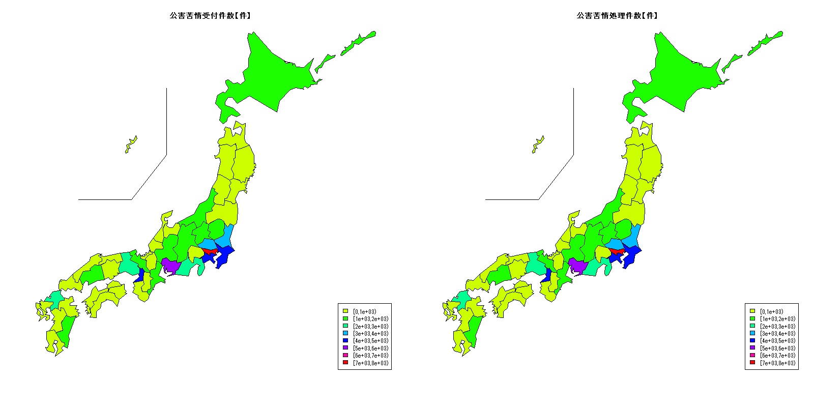
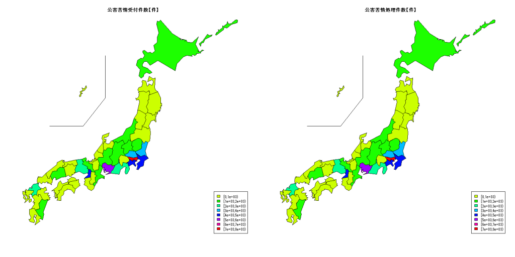
総務省統計局が発表している「都道府県・市区町村のすがた(社会・人口統計体系)」から、都道府県別の2017年の公害苦情受付件数【件】と公害苦情処理件数【件】を表示してみます。
| 都道府県 |
公害苦情受付件数 |
公害苦情処理件数 |
| 北海道 |
1491 |
1491 |
| 青森 |
494 |
494 |
| 岩手 |
526 |
526 |
| 宮城 |
640 |
640 |
| 秋田 |
355 |
355 |
| 山形 |
702 |
702 |
| 福島 |
604 |
604 |
| 茨城 |
3677 |
3677 |
| 栃木 |
1465 |
1465 |
| 群馬 |
1303 |
1303 |
| 埼玉 |
3546 |
3546 |
| 千葉 |
4794 |
4794 |
| 東京 |
7403 |
7403 |
| 神奈川 |
4427 |
4427 |
| 新潟 |
1023 |
1023 |
| 富山 |
322 |
322 |
| 石川 |
391 |
391 |
| 福井 |
612 |
612 |
| 山梨 |
692 |
692 |
| 長野 |
1907 |
1907 |
| 岐阜 |
1496 |
1496 |
| 静岡 |
2223 |
2223 |
| 愛知 |
5634 |
5634 |
| 三重 |
1245 |
1245 |
|
| 都道府県 |
公害苦情受付件数 |
公害苦情処理件数 |
| 滋賀 |
818 |
818 |
| 京都 |
1803 |
1803 |
| 大阪 |
4939 |
4939 |
| 兵庫 |
2292 |
2292 |
| 奈良 |
787 |
787 |
| 和歌山 |
801 |
801 |
| 鳥取 |
378 |
378 |
| 島根 |
292 |
292 |
| 岡山 |
873 |
873 |
| 広島 |
1253 |
1253 |
| 山口 |
698 |
698 |
| 徳島 |
475 |
475 |
| 香川 |
381 |
381 |
| 愛媛 |
855 |
855 |
| 高知 |
300 |
300 |
| 福岡 |
2981 |
2981 |
| 佐賀 |
350 |
350 |
| 長崎 |
973 |
973 |
| 熊本 |
786 |
786 |
| 大分 |
805 |
805 |
| 宮崎 |
1063 |
1063 |
| 鹿児島 |
967 |
967 |
| 沖縄 |
842 |
842 |
|
|
library(leaflet)
library(knitr)
library(kableExtra)
library(dplyr)
library(tidyr)
library(stringr)

dat <- read.csv("http://www.dinov.tokyo/Data/JP_Pref/Pref_data.csv", header = TRUE, fileEncoding="UTF-8")
col_start <- 0.2
col_end <- 0.0


table_df<-data.frame(都道府県=dat$都道府県, 公害苦情受付件数=dat$公害苦情受付件数, 公害苦情処理件数=dat$公害苦情処理件数)

datc_k <- cut(dat$公害苦情受付件数, hist(dat$公害苦情受付件数, plot=FALSE)$breaks, right=FALSE)
datc_kcol <- rainbow(length(levels(datc_k)), start = col_start, end=col_end)[as.integer(datc_k)]
datc_m <- cut(dat$公害苦情処理件数, hist(dat$公害苦情処理件数, plot=FALSE)$breaks, right=FALSE)
datc_mcol <- rainbow(length(levels(datc_m)), start = col_start, end=col_end)[as.integer(datc_m)]

library(NipponMap)
windowsFonts(JP4=windowsFont("Biz Gothic"))
windows(width=1600, height=800)

png("0plot1.png", width = 1600, height = 800)
par(family="JP4")
layout(matrix(1:2, 1, 2))
JapanPrefMap(datc_kcol, main="公害苦情受付件数【件】")
legend("bottomright", fill=rainbow(length(levels(datc_k)), start = col_start, end=col_end), legend=names(table(datc_k)))
JapanPrefMap(datc_mcol, main="公害苦情処理件数【件】")
legend("bottomright", fill=rainbow(length(levels(datc_m)), start = col_start, end=col_end), legend=names(table(datc_m)))
dev.off()

library(clipr)
t1=kable(table_df[c(1:24),], align = "c", row.names=FALSE) %>%
  kable_styling(full_width = F) %>%
  column_spec(1, bold = T) %>%
  collapse_rows(columns = 1, valign = "middle")
t2=kable(table_df[c(25:47),], align = "c", row.names=FALSE) %>%
  kable_styling(full_width = F) %>%
  column_spec(1, bold = T) %>%
  collapse_rows(columns = 1, valign = "middle")
paste(c('<table><tr valign="top"><td>', t1, '</td><td>', t2, '</td><tr></table>'), sep = '') %>% write_clip