【R】Time Series Machine Learning
1. はじめに
時系列データの機械学習をしてみます。timetkというパッケージを使います。データは、UCI Machine Learning Repositoryからレンタルバイクのデータを利用します。こちらのtimetikeのVignetteを参考にしました。
2. データ
2.1 準備
必要なパッケージを読み込みます。
library(tidymodels)
library(modeltime)
library(tidyverse)
library(timetk)

interactive = TRUE #Plotをインタラクティブに
2.2 データ
データは、UCI Machine Learning RepositoryからBike Sharing Datasetを使用します。
Source: Fanaee-T, Hadi, and Gama, Joao, ‘Event labeling combining ensemble detectors and background knowledge’, Progress in Artificial Intelligence (2013): pp. 1-15, Springer Berlin Heidelberg
レンタルバイク事業で得られたデータです。今回は、日付dtedayと貸出数cntを用います。
bike_transactions_tbl <- bike_sharing_daily %>%
  select(dteday, cnt) %>%
  set_names(c("date", "value"))

bike_transactions_tbl
> bike_transactions_tbl
# A tibble: 731 x 2
   date       value
   <date>     <dbl>
 1 2011-01-01   985
 2 2011-01-02   801
 3 2011-01-03  1349
 4 2011-01-04  1562
 5 2011-01-05  1600
 6 2011-01-06  1606
 7 2011-01-07  1510
 8 2011-01-08   959
 9 2011-01-09   822
10 2011-01-10  1321
# ... with 721 more rows
2.3 データの確認
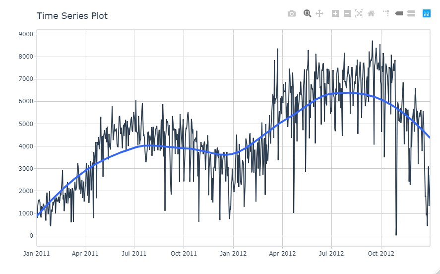
データをプロットして確認します。plot_time_series関数で時系列データとしてプロットします。interactive=FALSEにすると、インタラクティブではなく、ggplotのプロットとなります。トレンドと周期性とノイズが程よく入っているデータっぽいですね。
bike_transactions_tbl %>%
  plot_time_series(date, value, .interactive = interactive)
3. 機械学習
3.1 データ準備
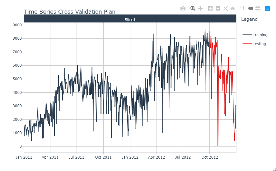
学習用とテスト用のデータを準備します。3か月分をテスト用とします(assess=”3 months”)。
splits <- bike_transactions_tbl %>%
  time_series_split(assess = "3 months", cumulative = TRUE)
学習用/テスト用データをプロットして確認します。
splits %>%
  tk_time_series_cv_plan() %>% #dataframeに変換
  plot_time_series_cv_plan(date, value, .interactive = interactive) #データをプロット
3.2 モデリング
目的変数をvalueとしてrecipeを作ります。timetkパッケージでは機械学習をサポートしてくれるstep_timeseries_signature()という関数があります。
recipe_spec_timeseries <- recipe(value ~ ., data = training(splits)) %>%
    step_timeseries_signature(date)
bakeして機械学習に必要なデータセットを生成します。
bake(prep(recipe_spec_timeseries), new_data = training(splits))
> bake(prep(recipe_spec_timeseries), new_data = training(splits))
# A tibble: 641 x 29
   date       value date_index.num date_year date_year.iso date_half date_quarter date_month date_month.xts
   <date>     <dbl>          <int>     <int>         <int>     <int>        <int>      <int>          <int>
 1 2011-01-01   985     1293840000      2011          2010         1            1          1              0
 2 2011-01-02   801     1293926400      2011          2010         1            1          1              0
 3 2011-01-03  1349     1294012800      2011          2011         1            1          1              0
 4 2011-01-04  1562     1294099200      2011          2011         1            1          1              0
 5 2011-01-05  1600     1294185600      2011          2011         1            1          1              0
 6 2011-01-06  1606     1294272000      2011          2011         1            1          1              0
 7 2011-01-07  1510     1294358400      2011          2011         1            1          1              0
 8 2011-01-08   959     1294444800      2011          2011         1            1          1              0
 9 2011-01-09   822     1294531200      2011          2011         1            1          1              0
10 2011-01-10  1321     1294617600      2011          2011         1            1          1              0
# ... with 631 more rows, and 20 more variables: date_month.lbl <ord>, date_day <int>, date_hour <int>,
#   date_minute <int>, date_second <int>, date_hour12 <int>, date_am.pm <int>, date_wday <int>, date_wday.xts <int>,
#   date_wday.lbl <ord>, date_mday <int>, date_qday <int>, date_yday <int>, date_mweek <int>, date_week <int>,
#   date_week.iso <int>, date_week2 <int>, date_week3 <int>, date_week4 <int>, date_mday7 <int>
recipe_spec_final <- recipe_spec_timeseries %>%
step_fourier(date, period = 365, K = 5) %>%
step_rm(date) %>%
step_rm(contains("iso"), contains("minute"), contains("hour"),
contains("am.pm"), contains("xts")) %>%
step_normalize(contains("index.num"), date_year) %>%
step_dummy(contains("lbl"), one_hot = TRUE)
juice(prep(recipe_spec_final))
> juice(prep(recipe_spec_final))
# A tibble: 641 x 47
   value date_index.num date_year date_half date_quarter date_month date_day date_second date_wday date_mday date_qday
   <dbl>          <dbl>     <dbl>     <int>        <int>      <int>    <int>       <int>     <int>     <int>     <int>
 1   985          -1.73    -0.869         1            1          1        1           0         7         1         1
 2   801          -1.72    -0.869         1            1          1        2           0         1         2         2
 3  1349          -1.72    -0.869         1            1          1        3           0         2         3         3
 4  1562          -1.71    -0.869         1            1          1        4           0         3         4         4
 5  1600          -1.71    -0.869         1            1          1        5           0         4         5         5
 6  1606          -1.70    -0.869         1            1          1        6           0         5         6         6
 7  1510          -1.70    -0.869         1            1          1        7           0         6         7         7
 8   959          -1.69    -0.869         1            1          1        8           0         7         8         8
 9   822          -1.68    -0.869         1            1          1        9           0         1         9         9
10  1321          -1.68    -0.869         1            1          1       10           0         2        10        10
# ... with 631 more rows, and 36 more variables: date_yday <int>, date_mweek <int>, date_week <int>,
#   date_week2 <int>, date_week3 <int>, date_week4 <int>, date_mday7 <int>, date_sin365_K1 <dbl>,
#   date_cos365_K1 <dbl>, date_sin365_K2 <dbl>, date_cos365_K2 <dbl>, date_sin365_K3 <dbl>, date_cos365_K3 <dbl>,
#   date_sin365_K4 <dbl>, date_cos365_K4 <dbl>, date_sin365_K5 <dbl>, date_cos365_K5 <dbl>, date_month.lbl_01 <dbl>,
#   date_month.lbl_02 <dbl>, date_month.lbl_03 <dbl>, date_month.lbl_04 <dbl>, date_month.lbl_05 <dbl>,
#   date_month.lbl_06 <dbl>, date_month.lbl_07 <dbl>, date_month.lbl_08 <dbl>, date_month.lbl_09 <dbl>,
#   date_month.lbl_10 <dbl>, date_month.lbl_11 <dbl>, date_month.lbl_12 <dbl>, date_wday.lbl_1 <dbl>,
#   date_wday.lbl_2 <dbl>, date_wday.lbl_3 <dbl>, date_wday.lbl_4 <dbl>, date_wday.lbl_5 <dbl>,
#   date_wday.lbl_6 <dbl>, date_wday.lbl_7 <dbl>
モデルを指定します。今回は、線形回帰とします。
model_spec_lm <- linear_reg(mode = "regression") %>%
    set_engine("lm")
レシピとモデルを決めたので、ワークフローを設定します。
workflow_lm <- workflow() %>%
    add_recipe(recipe_spec_final) %>%
    add_model(model_spec_lm)

workflow_lm
> workflow_lm
== Workflow ====================================================================
Preprocessor: Recipe
Model: linear_reg()

-- Preprocessor ----------------------------------------------------------------
6 Recipe Steps

* step_timeseries_signature()
* step_fourier()
* step_rm()
* step_rm()
* step_normalize()
* step_dummy()

-- Model -----------------------------------------------------------------------
Linear Regression Model Specification (regression)

Computational engine: lm
学習します。
workflow_fit_lm <- workflow_lm %>% fit(data = training(splits))
3.3 予測
modeltimeパッケージを使って、予測します。
model_table <- modeltime_table(
  workflow_fit_lm
)

model_table
> model_table
# Modeltime Table
# A tibble: 1 x 3
  .model_id .model     .model_desc
      <int> <list>     <chr>
1         1 <workflow> LM
キャリブレーション
calibration_table <- model_table %>%
  modeltime_calibrate(testing(splits))

calibration_table
> calibration_table
# Modeltime Table
# A tibble: 1 x 5
.model_id .model .model_desc .type .calibration_data
<int> <list> <chr> <chr> <list>
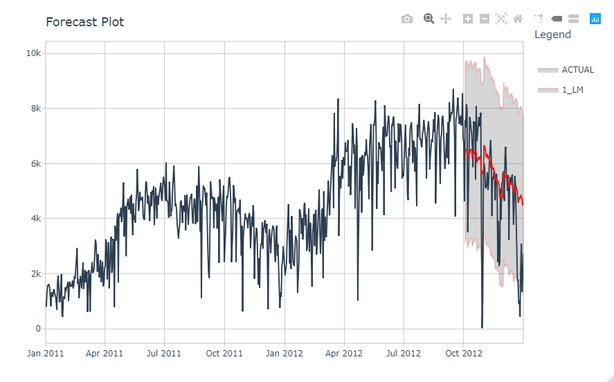
1 1 <workflow> LM Test <tibble [90 x 4]>テスト用データで予測してみます。
calibration_table %>%
  modeltime_forecast(actual_data = bike_transactions_tbl) %>%
  plot_modeltime_forecast(.interactive = interactive)
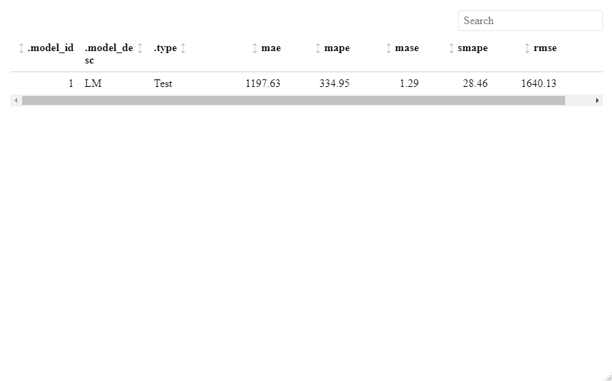
予測精度(テスト用データ)を見てみます。
calibration_table %>%
  modeltime_accuracy() %>%
  table_modeltime_accuracy(.interactive = interactive)
最後に、4年後(=48months)までの予測をしてみます。
calibration_table %>%
  modeltime_refit(bike_transactions_tbl) %>%
  modeltime_forecast(h = "48 months", actual_data = bike_transactions_tbl) %>%
  plot_modeltime_forecast(.interactive = interactive)
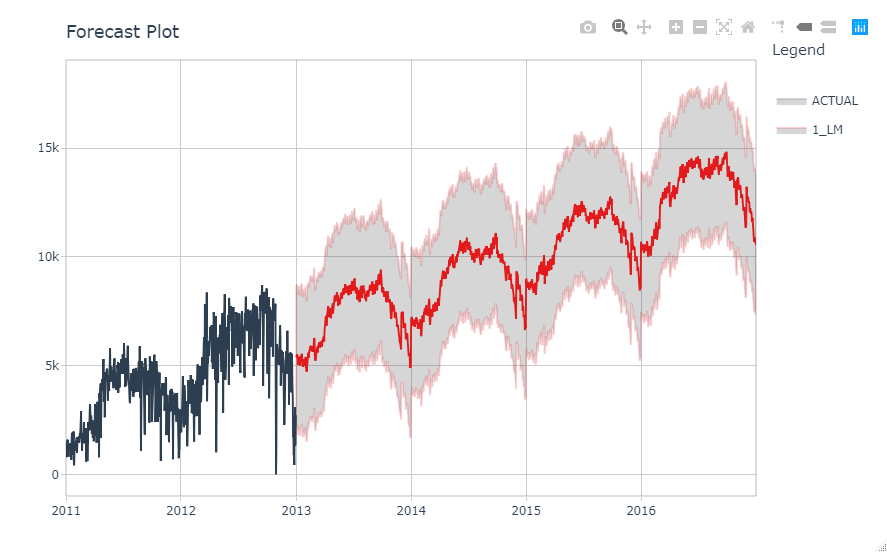
なんだか、それらしい予測データとなっています。
4. さいごに
timetkパッケージとmodeltimeパッケージを使って、時系列データの機械学習をしてみました。今後、活用していきたいです。