【R】Tidymodelsで機械学習
1. はじめに
Tidymodelsを使って、機械学習をしてみます。
2. データ
データは、UCI Machine Learning Repositoryから、David J. SlateによるLetter Recognition Data Setを使います。これは、A~Zの26文字のアルファベットのグリフの属性(縦横サイズ比、ピクセルの割合、縦横位置等)が示されたデータです。その属性から文字を認識させることが、今回の目的となります。
このデータには、20,000件のインスタンスが含まれています。データをダウンロードして、読み込みます。目的のlettrはファクター型にしておきます。
library(tidyverse)
library(tidymodels)

dat <- read.csv("letter-recognition.csv", header = TRUE)

dat2 <- dat %>% mutate(lettr = factor(dat$lettr))
str(dat2)
> str(dat2)
'data.frame':	20000 obs. of  17 variables:
 $ lettr: Factor w/ 26 levels "A","B","C","D",..: 20 9 4 14 7 19 2 1 10 13 ...
 $ x.box: int  2 5 4 7 2 4 4 1 2 11 ...
 $ y.box: int  8 12 11 11 1 11 2 1 2 15 ...
 $ width: int  3 3 6 6 3 5 5 3 4 13 ...
 $ high : int  5 7 8 6 1 8 4 2 4 9 ...
 $ onpix: int  1 2 6 3 1 3 4 1 2 7 ...
 $ x.bar: int  8 10 10 5 8 8 8 8 10 13 ...
 $ y.bar: int  13 5 6 9 6 8 7 2 6 2 ...
 $ x2bar: int  0 5 2 4 6 6 6 2 2 6 ...
 $ y2bar: int  6 4 6 6 6 9 6 2 6 2 ...
 $ xybar: int  6 13 10 4 6 5 7 8 12 12 ...
 $ x2ybr: int  10 3 3 4 5 6 6 2 4 1 ...
 $ xy2br: int  8 9 7 10 9 6 6 8 8 9 ...
 $ x.ege: int  0 2 3 6 1 0 2 1 1 8 ...
 $ xegvy: int  8 8 7 10 7 8 8 6 6 1 ...
 $ y.ege: int  0 4 3 2 5 9 7 2 1 1 ...
 $ yegvx: int  8 10 9 8 10 7 10 7 7 8 ...
訓練用データとテスト用データを用意します。
lettr_split <- initial_split(dat2, strata = lettr, prop = 0.9)
lettr_train <- training(lettr_split)
lettr_test <- testing(lettr_split)
クロスバリデーションの準備をします。
set.seed(123)

lettr_folds <-
  vfold_cv(lettr_train, v=10, strata=lettr)
3. モデル
モデルを定義します。今回は、決定木を使い、engineはrpartにて分類します。
tree_mod <-
  decision_tree() %>%
  set_engine(engine = "rpart") %>%
  set_mode("classification")
4. ワークフロー
ワークフローを定義します。
tree_wf <-
  workflow() %>%
  add_formula(lettr ~.) %>%
  add_model(tree_mod)
5. モデルの学習
学習してみます。
tree_wf %>%
  fit_resamples(resamples = lettr_folds) %>%
  collect_metrics(summarize = FALSE)
> tree_wf %>%
+   fit_resamples(resamples = lettr_folds) %>%
+   collect_metrics(summarize = FALSE)
# A tibble: 20 x 4
   id     .metric  .estimator .estimate
   <chr>  <chr>    <chr>          <dbl>
 1 Fold01 accuracy multiclass     0.462
 2 Fold01 roc_auc  hand_till      0.900
 3 Fold02 accuracy multiclass     0.498
 4 Fold02 roc_auc  hand_till      0.906
 5 Fold03 accuracy multiclass     0.472
 6 Fold03 roc_auc  hand_till      0.903
 7 Fold04 accuracy multiclass     0.482
 8 Fold04 roc_auc  hand_till      0.903
 9 Fold05 accuracy multiclass     0.492
10 Fold05 roc_auc  hand_till      0.908
11 Fold06 accuracy multiclass     0.463
12 Fold06 roc_auc  hand_till      0.899
13 Fold07 accuracy multiclass     0.473
14 Fold07 roc_auc  hand_till      0.905
15 Fold08 accuracy multiclass     0.476
16 Fold08 roc_auc  hand_till      0.903
17 Fold09 accuracy multiclass     0.486
18 Fold09 roc_auc  hand_till      0.902
19 Fold10 accuracy multiclass     0.481
20 Fold10 roc_auc  hand_till      0.903
6. チューニング
ここで、パラメータのチューニングをしてみます。今度は、ランダムフォレストを使ってみます。
まず、モデルを定義します。チューニングするパラメータは、mtryとmin_nとします。rangerをエンジンとして分類します。
rf_tuner <-
  rand_forest(
    mtry = tune(),
    min_n = tune()
  ) %>%
  set_engine(engine = "ranger") %>%
  set_mode("classification")
ワークフローのモデルをアップデートします。
rf_wf <-
  tree_wf %>%
  update_model(rf_tuner)
tune_gridでチューニングを実行します。
set.seed(213)
rf_results <-
  rf_wf %>%
  tune_grid(resamples = lettr_folds,
            metrics = metric_set(roc_auc))
結果を表示してみます。
rf_results %>% collect_metrics()
> rf_results %>% collect_metrics()
# A tibble: 10 x 8
    mtry min_n .metric .estimator  mean     n   std_err .config
   <int> <int> <chr>   <chr>      <dbl> <int>     <dbl> <chr>
 1     7    35 roc_auc hand_till  0.999    10 0.0000537 Model01
 2     6    15 roc_auc hand_till  0.999    10 0.0000409 Model02
 3     2     2 roc_auc hand_till  1.00     10 0.0000297 Model03
 4    13    12 roc_auc hand_till  0.999    10 0.0000434 Model04
 5     9    28 roc_auc hand_till  0.999    10 0.0000541 Model05
 6    13    23 roc_auc hand_till  0.999    10 0.0000598 Model06
 7     4    40 roc_auc hand_till  0.999    10 0.0000609 Model07
 8     4    29 roc_auc hand_till  0.999    10 0.0000481 Model08
 9    15     8 roc_auc hand_till  0.999    10 0.0000603 Model09
10    11    19 roc_auc hand_till  0.999    10 0.0000440 Model10
決定木よりもランダムフォレストの方が結果がよさそうです。どのモデルが良いかわかりやすく表示させるために、良い順に表示させます。
rf_results %>%
  show_best(metric = "roc_auc", n=4)
> rf_results %>%
+   show_best(metric = "roc_auc", n=4)
# A tibble: 4 x 8
   mtry min_n .metric .estimator  mean     n   std_err .config
  <int> <int> <chr>   <chr>      <dbl> <int>     <dbl> <chr>
1     2     2 roc_auc hand_till  1.00     10 0.0000297 Model03
2     6    15 roc_auc hand_till  0.999    10 0.0000409 Model02
3    13    12 roc_auc hand_till  0.999    10 0.0000434 Model04
4    11    19 roc_auc hand_till  0.999    10 0.0000440 Model10
mtry=2, min_n=2が最も良かったようです。
rf_results %>%
  autoplot()
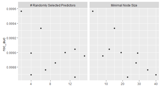
図示すると一目瞭然です。
最も良いモデルを選択して、ファイナライズします。
lettr_best <-
  rf_results %>%
  select_best(metric = "roc_auc")

last_rf_workflow <-
  rf_wf %>%
  finalize_workflow(lettr_best)

last_rf_fit <-
  last_rf_workflow %>%
  last_fit(split = lettr_split)
結果を見ますと。
last_rf_fit %>%
  collect_metrics()
> last_rf_fit %>%
+   collect_metrics()
# A tibble: 2 x 3
  .metric  .estimator .estimate
  <chr>    <chr>          <dbl>
1 accuracy multiclass     0.966
2 roc_auc  hand_till      1.00
すごくいいですね!
予測させた結果を見てみますと。
ret <- last_rf_fit %>%
  collect_predictions()
rslt <- data.frame(ret$lettr, ret$.pred_class)
head(rslt, 20)
> head(rslt, 20)
   ret.lettr ret..pred_class
1          I               I
2          D               D
3          B               B
4          M               M
5          H               H
6          B               B
7          P               P
8          G               G
9          G               G
10         L               L
11         Q               Q
12         V               V
13         S               S
14         U               U
15         P               P
16         A               A
17         A               A
18         Y               Y
19         B               H
20         V               V
データを見ても、正確に予測できています。
7. さいごに
少しずつですが、Tidymodelsの使い方もわかってきました。でも、まだまだ経験を積まないと。。。
