【R】Kerasを使ってみる(Fashion MNIST)
2020年10月2日
1. はじめに
どんどん、Kerasを使って、なるべく早く慣れたいと思います。今回は、Fashion MNISTを使って画像の分類を行います。Tensorflow with Rのtutorialをやってみました。
2. 使ってみる。
2.1 データ準備
Fashion MNISTデータセットは、10種類の洋服に関して28×28ピクセルのRGBカラーイメージが60,000レコード入っています。
| Digit | Class |
|---|---|
| 0 | T-shirt/top |
| 1 | Trouser |
| 2 | Pullover |
| 3 | Dress |
| 4 | Coat |
| 5 | Sandal |
| 6 | Shirt |
| 7 | Sneaker |
| 8 | Bag |
| 9 | Ankle boot |
library(keras)

fashion_mnist <- dataset_fashion_mnist()
データが大きいので、読み込むまでに少し時間がかかります。
str(fashion_mnist)
> str(fashion_mnist)
List of 2
 $ train:List of 2
  ..$ x: int [1:60000, 1:28, 1:28] 0 0 0 0 0 0 0 0 0 0 ...
  ..$ y: int [1:60000(1d)] 9 0 0 3 0 2 7 2 5 5 ...
 $ test :List of 2
  ..$ x: int [1:10000, 1:28, 1:28] 0 0 0 0 0 0 0 0 0 0 ...
  ..$ y: int [1:10000(1d)] 9 2 1 1 6 1 4 6 5 7 ...
データはすでに学習用とテスト用に分かれています。それぞれを変数に格納してあげます。
c(train_images, train_labels) %<-% fashion_mnist$train
c(test_images, test_labels) %<-% fashion_mnist$test

class_names = c('T-shirt/top',
                'Trouser',
                'Pullover',
                'Dress',
                'Coat',
                'Sandal',
                'Shirt',
                'Sneaker',
                'Bag',
                'Ankle boot')

dim(train_images)
dim(train_labels)
> dim(train_images)
[1] 60000    28    28
> dim(train_labels)
[1] 60000ggplotにて、最初のイメージを表示してみます。
library(tidyverse)
library(ggplot2)

image_1 <- as.data.frame(train_images[1, , ])
colnames(image_1) <- seq_len(ncol(image_1))
image_1$y <- seq_len(nrow(image_1))
image_1 <- gather(image_1, "x", "value", -y)
image_1$x <- as.integer(image_1$x)

ggplot(image_1, aes(x = x, y = y, fill = value)) +
  geom_tile() +
  scale_fill_gradient(low = "white", high = "black", na.value = NA) +
  scale_y_reverse() +
  theme_minimal() +
  theme(panel.grid = element_blank())   +
  theme(aspect.ratio = 1) +
  xlab("") +
  ylab("")
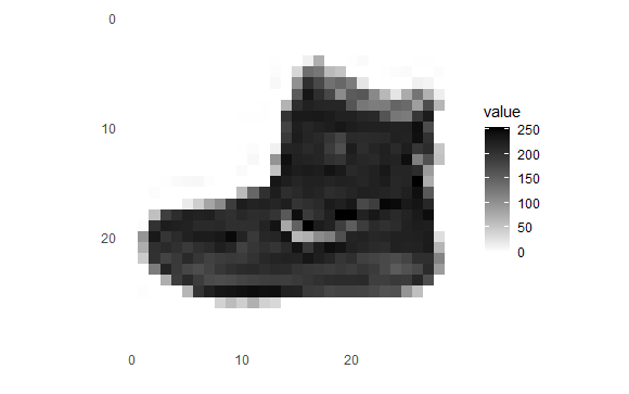
はい、ブーツです。
画像は、256諧調ですが、精度よく学習できるように0~1へ直してあげます。
train_images <- train_images / 255
test_images <- test_images / 255
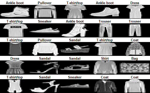
25個の画像を見てみます。
par(mfcol=c(5,5))
par(mar=c(0, 0, 1.5, 0), xaxs='i', yaxs='i')
for (i in 1:25) {
  img <- train_images[i, , ]
  img <- t(apply(img, 2, rev))
  image(1:28, 1:28, img, col = gray((0:255)/255), xaxt = 'n', yaxt = 'n',
        main = paste(class_names[train_labels[i] + 1]))
}
2.2 モデル構築
次にモデルを作ります。入力は、28×28ピクセルです。出力は、分類ですのでsoftmaxにします。
model <- keras_model_sequential()
model %>%
  layer_flatten(input_shape = c(28, 28)) %>%
  layer_dense(units = 128, activation = 'relu') %>%
  layer_dense(units = 10, activation = 'softmax')
コンパイルします。
model %>% compile(
  optimizer = 'adam',
  loss = 'sparse_categorical_crossentropy',
  metrics = c('accuracy')
)
2.3 学習・評価
では、実際に学習してみます。
model %>% fit(train_images, train_labels, epochs = 5, verbose = 2)
> model %>% fit(train_images, train_labels, epochs = 5, verbose = 2)
Train on 60000 samples
Epoch 1/5
60000/60000 - 4s - loss: 4.3115 - accuracy: 0.7157
Epoch 2/5
60000/60000 - 4s - loss: 0.8543 - accuracy: 0.7385
Epoch 3/5
60000/60000 - 4s - loss: 0.7480 - accuracy: 0.7573
Epoch 4/5
60000/60000 - 4s - loss: 0.6727 - accuracy: 0.7815
Epoch 5/5
60000/60000 - 4s - loss: 0.6246 - accuracy: 0.7920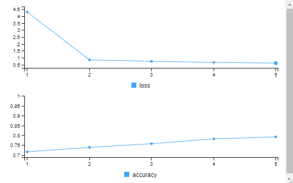
結果はどうでしょう?
score <- model %>% evaluate(test_images, test_labels, verbose = 0)

cat('Test loss:', score$loss, "\n")

cat('Test accuracy:', score$acc, "\n")
> cat('Test loss:', score$loss, "\n")
Test loss: 0.7543408
>
> cat('Test accuracy:', score$acc, "\n")
Test accuracy: 0.777
この結果はどうなんでしょうか?まあまあ、いいのでしょうか?
モデルの保存と呼び出しは次の通りです。
model %>% save_model_tf("model_fashionMNIST_trained")
new_model <- load_model_tf("model_fashionMNIST_trained")
2.4 予測
テストデータで予測してみます。
predictions_newModel <- new_model %>% predict(test_images)
predictions_newModel[1, ]
> predictions[1, ]
 [1] 0 0 0 0 0 0 0 0 0 1
最初のデータはブーツですね。次のように調べても良いです。
which.max(predictions[1, ])
> which.max(predictions[1, ])
[1] 10
正解は?
test_labels[1]
> test_labels[1]
[1] 9
はい、9番のブーツであってます!
予測したラベルを全部見てみます。
class_pred <- model %>% predict_classes(test_images)
class_pred[1:nrow(predictions)]
> class_pred[1:nrow(predictions)]
   [1] 9 2 1 1 6 1 4 2 5 7 4 5 5 3 4 1 2 4 0 0 0 7 7 5 1 2 2 3 9 3 8 8 3 3 8 0 7 5 7 9 0
  [42] 1 6 7 2 7 6 1 4 6 2 2 5 0 4 2 8 4 8 0 7 7 8 5 1 1 0 6 7 8 7 0 0 0 4 3 1 2 8 4 1 8
  [83] 5 9 5 0 3 4 0 6 5 6 2 7 1 8 0 1 6 2 3 4 7 2 7 8 5 7 9 4 2 5 7 0 5 2 8 6 7 0 0 0 9
 [124] 9 3 0 8 4 1 5 4 1 9 1 8 2 2 1 2 5 1 0 0 0 1 0 1 3 2 6 6 6 1 3 5 0 4 7 9 3 7 2 3 9
 [165] 0 9 4 7 4 2 0 5 4 1 2 1 3 0 9 1 0 9 6 0 7 5 9 4 4 7 1 2 1 4 3 2 0 3 2 1 1 0 2 9 2
 [206] 4 0 7 9 8 4 1 0 4 1 3 1 6 7 4 8 5 6 0 7 7 0 2 7 0 7 8 9 4 9 0 5 1 4 2 5 6 9 2 4 0
 [247] 2 4 2 4 9 7 6 5 5 4 8 5 4 3 0 4 8 2 0 2 6 0 9 0 1 6 0 4 3 0 8 3 7 4 0 1 2 6 0 4 0
 [288] 7 5 6 5 9 5 0 5 5 1 9 8 3 3 3 2 8 0 0 2 9 7 7 1 3 0 4 2 4 7 1 2 4 8 2 0 5 4 2 7 7
 [329] 7 3 3 7 0 7 1 3 7 0 2 3 4 0 3 1 0 1 9 4 9 9 1 7 0 3 0 0 6 4 8 0 1 4 2 4 4 7 3 4 2
 [370] 5 0 7 9 4 0 9 3 9 0 2 5 0 0 3 5 8 1 0 2 0 6 4 7 5 2 0 4 6 1 2 0 9 7 0 6 4 0 0 4 3
 [411] 0 2 7 6 9 4 2 1 5 4 5 3 8 5 8 4 4 8 9 8 6 2 4 4 6 4 1 2 1 3 0 7 8 8 4 5 3 1 7 5 3
 [452] 3 0 1 2 2 9 4 0 6 4 4 2 0 0 6 3 8 2 8 9 4 0 7 0 6 6 9 2 9 7 9 3 7 5 7 8 1 0 0 0 4
 [493] 8 9 7 9 1 2 7 3 6 0 5 7 1 8 6 2 6 2 4 2 0 1 9 8 5 1 9 1 2 8 3 8 9 2 4 6 8 0 2 0 5
 [534] 8 8 5 3 9 4 3 4 4 7 1 0 1 4 0 4 9 6 1 5 1 1 1 9 3 4 5 1 0 4 6 4 0 0 5 8 0 6 4 6 7
 [575] 7 8 9 3 0 2 7 0 7 9 3 4 0 0 5 0 1 1 5 9 3 2 5 7 8 1 2 9 7 7 1 0 9 6 4 9 0 7 6 8 2
 [616] 7 3 2 3 0 2 4 0 7 3 0 7 8 0 2 9 4 1 0 4 4 0 4 4 4 7 5 8 4 9 1 0 5 4 4 4 0 0 4 5 6
 [657] 0 6 5 4 1 0 1 3 4 4 3 8 2 0 0 7 0 4 6 8 5 0 8 2 9 0 8 9 6 4 4 9 6 4 5 0 9 5 3 4 2
 [698] 8 3 3 8 3 4 0 9 7 7 4 8 9 1 3 7 3 0 2 4 7 1 0 0 8 7 2 6 4 6 4 1 5 9 2 0 1 6 7 2 0
 [739] 4 3 3 8 1 1 8 5 7 7 8 7 4 0 7 0 8 0 9 7 4 1 3 6 4 0 0 6 3 4 8 4 0 8 9 2 4 5 9 1 4
 [780] 4 9 2 1 7 9 0 8 3 7 7 1 1 1 6 9 5 3 8 4 4 9 0 8 3 2 2 4 7 1 4 9 3 5 8 5 4 7 4 8 5
 [821] 9 3 3 4 7 1 7 3 5 4 4 5 8 3 7 1 2 0 1 9 8 2 7 1 4 7 5 9 9 1 8 4 5 7 1 9 0 1 6 0 2
 [862] 1 7 1 1 5 7 1 5 2 4 3 3 1 1 4 9 4 3 7 7 0 8 9 9 2 1 1 2 0 3 5 9 2 0 5 5 1 5 7 8 7
 [903] 7 3 2 2 0 4 0 2 0 2 5 5 1 2 0 9 3 7 8 4 8 3 2 7 6 7 4 8 0 6 4 4 3 2 9 0 2 4 9 1 8
 [944] 1 7 5 5 6 0 2 1 0 5 6 0 0 6 7 5 0 0 5 9 4 8 2 0 4 0 2 9 0 7 7 1 4 2 0 7 0 9 9 8 8
 [985] 3 6 4 4 6 6 3 4 3 7 4 9 3 4 7 7
 [ reached getOption("max.print") -- omitted 9000 entries ]
今度は、予測の結果を画像で見てみます。最初の25個だけですが。正解だとラベルを緑で、不正解だと赤で表示します。
par(mfcol=c(5,5))
par(mar=c(0, 0, 1.5, 0), xaxs='i', yaxs='i')
for (i in 1:25) {
  img <- test_images[i, , ]
  img <- t(apply(img, 2, rev))
  predicted_label <- which.max(predictions[i, ]) - 1
  true_label <- test_labels[i]
  if (predicted_label == true_label) {
    color <- '#008800'
  } else {
    color <- '#bb0000'
  }
  image(1:28, 1:28, img, col = gray((0:255)/255), xaxt = 'n', yaxt = 'n',
        main = paste0(class_names[predicted_label + 1], " (",
                      class_names[true_label + 1], ")"),
        col.main = color)
}
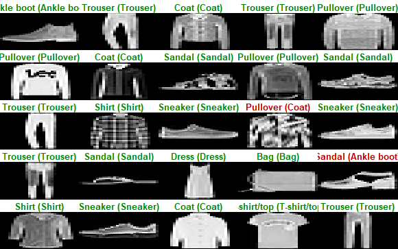
多くは表示できませんが、画像の方が理解しやすいですね。
confusion matrix を見てみます。
library("caret")
confusionMatrix(as.factor(class_pred[1:nrow(predictions)]),as.factor(test_labels))
> confusionMatrix(as.factor(class_pred[1:nrow(predictions)]),as.factor(test_labels))
Confusion Matrix and Statistics

          Reference
Prediction   0   1   2   3   4   5   6   7   8   9
         0 831  15  69  45   9   9 324   2 127   1
         1   5 952   3   6   0   0   2   0   0   0
         2  33   3 577   9 109   0 231   0   2   0
         3  52  19   6 812  22   0  20   0   5   0
         4   2   5 254  34 786   0 174   0   6   0
         5   0   0   0   1   0 877   0  12   0  35
         6  74   6  90  92  72   0 245   0  10   0
         7   0   0   0   0   0  81   0 976   6  94
         8   3   0   1   1   2   4   4   1 844   0
         9   0   0   0   0   0  29   0   9   0 870

Overall Statistics

               Accuracy : 0.777
                 95% CI : (0.7687, 0.7851)
    No Information Rate : 0.1
    P-Value [Acc > NIR] : < 2.2e-16

                  Kappa : 0.7522

 Mcnemar's Test P-Value : NA

Statistics by Class:

                     Class: 0 Class: 1 Class: 2 Class: 3 Class: 4 Class: 5 Class: 6
Sensitivity            0.8310   0.9520   0.5770   0.8120   0.7860   0.8770   0.2450
Specificity            0.9332   0.9982   0.9570   0.9862   0.9472   0.9947   0.9618
Pos Pred Value         0.5803   0.9835   0.5985   0.8675   0.6233   0.9481   0.4160
Neg Pred Value         0.9803   0.9947   0.9532   0.9793   0.9755   0.9864   0.9198
Prevalence             0.1000   0.1000   0.1000   0.1000   0.1000   0.1000   0.1000
Detection Rate         0.0831   0.0952   0.0577   0.0812   0.0786   0.0877   0.0245
Detection Prevalence   0.1432   0.0968   0.0964   0.0936   0.1261   0.0925   0.0589
Balanced Accuracy      0.8821   0.9751   0.7670   0.8991   0.8666   0.9358   0.6034
                     Class: 7 Class: 8 Class: 9
Sensitivity            0.9760   0.8440   0.8700
Specificity            0.9799   0.9982   0.9958
Pos Pred Value         0.8436   0.9814   0.9581
Neg Pred Value         0.9973   0.9829   0.9857
Prevalence             0.1000   0.1000   0.1000
Detection Rate         0.0976   0.0844   0.0870
Detection Prevalence   0.1157   0.0860   0.0908
Balanced Accuracy      0.9779   0.9211   0.9329
本当は、ここから詳しくモデルを評価して、パラメータのチューニングをしたりして・・・というのが、お仕事なのでしょうけど、Deep Learningに触れることが目的なので、ここまで。
