【R】Kerasを使ってみる(Boston housing)
2020年10月12日
1. はじめに
Kerasをどんどん使って、とりあえず慣れようとしてます。今回もTensorflowのtutorialから、Regressionをやってみます。
ここでは、離散ラベルを予測する分類ではなく、連続値を扱う回帰を行います。
2. 使ってみる
2.1 データ
データは、頻出するThe Boston Housing Prices datasetです。1970年代中盤のボストン近郊の住宅価格の中央値を、住宅の仕様や周囲の環境でまとめたものです。データとしては、比較的小さく学習用に404、テスト用に102の合計506のデータです。目的変数は、住宅価格です。
学習用、テスト用のデータをデータトラベルに分けて読み込みます。
library(tidyverse)
library(keras)
library(tfdatasets)

boston_housing <- dataset_boston_housing()
c(train_data, train_labels) %<-% boston_housing$train
c(test_data, test_labels) %<-% boston_housing$test
データは、13の項目からなっています。MEDVが目的変数(単位:$1,000)です。
    CRIM - per capita crime rate by town
    ZN - proportion of residential land zoned for lots over 25,000 sq.ft.
    INDUS - proportion of non-retail business acres per town.
    CHAS - Charles River dummy variable (1 if tract bounds river; 0 otherwise)
    NOX - nitric oxides concentration (parts per 10 million)
    RM - average number of rooms per dwelling
    AGE - proportion of owner-occupied units built prior to 1940
    DIS - weighted distances to five Boston employment centres
    RAD - index of accessibility to radial highways
    TAX - full-value property-tax rate per $10,000
    PTRATIO - pupil-teacher ratio by town
    B - 1000(Bk - 0.63)^2 where Bk is the proportion of blacks by town
    LSTAT - % lower status of the population
    MEDV - Median value of owner-occupied homes in $1000's
列に名前を付けて、データとラベルを合わせてtibbleにします。
column_names <- c('CRIM', 'ZN', 'INDUS', 'CHAS', 'NOX', 'RM', 'AGE',
                  'DIS', 'RAD', 'TAX', 'PTRATIO', 'B', 'LSTAT')

train_df <- train_data %>%
  as_tibble(.name_repair = "minimal") %>%
  setNames(column_names) %>%
  mutate(label = train_labels)

test_df <- test_data %>%
  as_tibble(.name_repair = "minimal") %>%
  setNames(column_names) %>%
  mutate(label = test_labels)
データを正規化します。tfdatasetsパッケージにあるfeature_specを使います。
spec <- feature_spec(train_df, label ~ . ) %>%
  step_numeric_column(all_numeric(), normalizer_fn = scaler_standard()) %>%
  fit()

spec
> spec
-- Feature Spec ----------------------------------------------------------------
A feature_spec with 13 steps.
Fitted: TRUE
-- Steps -----------------------------------------------------------------------
The feature_spec has 1 dense features.
StepNumericColumn: CRIM, ZN, INDUS, CHAS, NOX, RM, AGE, DIS, RAD, TAX, PTRATIO, B, LSTAT
-- Dense features --------------------------------------------------------------
layer <- layer_dense_features( feature_columns = dense_features(spec), dtype = tf$float32 ) layer(train_df)
2.2 モデルを作る
input <- layer_input_from_dataset(train_df %>% select(-label))

output <- input %>%
  layer_dense_features(dense_features(spec)) %>%
  layer_dense(units = 64, activation = "relu") %>%
  layer_dense(units = 64, activation = "relu") %>%
  layer_dense(units = 1)

model <- keras_model(input, output)

summary(model)
> summary(model)
Model: "model_3"
_________________________________________________________________________________________
Layer (type)                 Output Shape       Param #    Connected to
=========================================================================================
AGE (InputLayer)             [(None,)]          0
_________________________________________________________________________________________
B (InputLayer)               [(None,)]          0
_________________________________________________________________________________________
CHAS (InputLayer)            [(None,)]          0
_________________________________________________________________________________________
CRIM (InputLayer)            [(None,)]          0
_________________________________________________________________________________________
DIS (InputLayer)             [(None,)]          0
_________________________________________________________________________________________
INDUS (InputLayer)           [(None,)]          0
_________________________________________________________________________________________
LSTAT (InputLayer)           [(None,)]          0
_________________________________________________________________________________________
NOX (InputLayer)             [(None,)]          0
_________________________________________________________________________________________
PTRATIO (InputLayer)         [(None,)]          0
_________________________________________________________________________________________
RAD (InputLayer)             [(None,)]          0
_________________________________________________________________________________________
RM (InputLayer)              [(None,)]          0
_________________________________________________________________________________________
TAX (InputLayer)             [(None,)]          0
_________________________________________________________________________________________
ZN (InputLayer)              [(None,)]          0
_________________________________________________________________________________________
dense_features_7 (DenseFeatu (None, 13)         0          AGE[0][0]
                                                           B[0][0]
                                                           CHAS[0][0]
                                                           CRIM[0][0]
                                                           DIS[0][0]
                                                           INDUS[0][0]
                                                           LSTAT[0][0]
                                                           NOX[0][0]
                                                           PTRATIO[0][0]
                                                           RAD[0][0]
                                                           RM[0][0]
                                                           TAX[0][0]
                                                           ZN[0][0]
_________________________________________________________________________________________
dense_9 (Dense)              (None, 64)         896        dense_features_7[0][0]
_________________________________________________________________________________________
dense_10 (Dense)             (None, 64)         4160       dense_9[0][0]
_________________________________________________________________________________________
dense_11 (Dense)             (None, 1)          65         dense_10[0][0]
=========================================================================================
Total params: 5,121
Trainable params: 5,121
Non-trainable params: 0
_________________________________________________________________________________________
コンパイルします。
model %>%
  compile(
    loss = "mse",
    optimizer = optimizer_rmsprop(),
    metrics = list("mean_absolute_error")
  )
学習はMAEで評価することにします。
モデルを再利用可能にするため、関数にしておきます。
build_model <- function() {
  input <- layer_input_from_dataset(train_df %>% select(-label))

  output <- input %>%
    layer_dense_features(dense_features(spec)) %>%
    layer_dense(units = 64, activation = "relu") %>%
    layer_dense(units = 64, activation = "relu") %>%
    layer_dense(units = 1)

  model <- keras_model(input, output)

  model %>%
    compile(
      loss = "mse",
      optimizer = optimizer_rmsprop(),
      metrics = list("mean_absolute_error")
    )

  model
}
2.3 学習
500エポックで学習します。学習とバリデーション精度をhistoryオブジェクトに保存します。経過を可視化するために、エポックが終わるごとにドットを表示するようにします。
print_dot_callback <- callback_lambda(
  on_epoch_end = function(epoch, logs) {
    if (epoch %% 80 == 0) cat("\n")
    cat(".")
  }
)

model <- build_model()

history <- model %>% fit(
  x = train_df %>% select(-label),
  y = train_df$label,
  epochs = 500,
  validation_split = 0.2,
  verbose = 0,
  callbacks = list(print_dot_callback)
)
................................................................................
................................................................................
................................................................................
................................................................................
................................................................................
................................................................................
....................
library(ggplot2) plot(history)
結果を表示してみます。
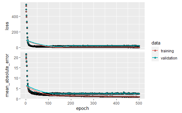
グラフから200エポック以降は、maeがほとんど向上しません。学習が終わった時点で自動的に学習を止めるようにしてみます。
early_stop <- callback_early_stopping(monitor = "val_loss", patience = 20)

model <- build_model()

history <- model %>% fit(
  x = train_df %>% select(-label),
  y = train_df$label,
  epochs = 500,
  validation_split = 0.2,
  verbose = 0,
  callbacks = list(early_stop)
)

plot(history)
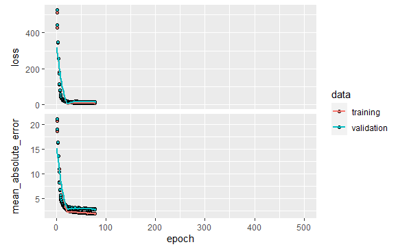
100エポック前で終了しています。
c(loss, mae) %<-% (model %>% evaluate(test_df %>% select(-label), test_df$label, verbose = 0))

paste0("Mean absolute error on test set: $", sprintf("%.2f", mae * 1000))
paste0("Loss : $", sprintf("%.2f", loss))
> paste0("Mean absolute error on test set: $", sprintf("%.2f", mae * 1000))
[1] "Mean absolute error on test set: $3372.70"
> paste0("Loss : $", sprintf("%.2f", loss))
[1] "Loss : $29.61"
2.4 予測
学習した結果を用いて、住宅価格を予測してみます。
test_predictions <- model %>% predict(test_df %>% select(-label))
test_predictions[ , 1]
 >test_predictions[ , 1]
  [1]  8.679926 17.808245 19.691261 30.397329 24.332861 18.431540 25.050531 20.281782
  [9] 18.619127 22.361448 15.843100 16.171593 14.411268 40.925022 19.873802 19.064783
 [17] 25.202995 19.877954 19.053623 40.360294 11.144051 16.264927 19.325394 14.044344
 [25] 20.190037 24.387886 30.155615 27.581944 11.066998 19.929132 18.255713 14.453447
 [33] 33.805740 23.609915 18.182421  8.101769 14.814152 17.369606 20.267996 23.970438
 [41] 28.117958 26.321718 15.065187 40.011372 29.142263 23.958763 25.803492 15.434764
 [49] 24.433462 21.044039 32.251938 19.035295 12.568875 15.159834 33.011894 26.719646
 [57] 13.318023 47.174225 34.385036 22.876797 26.065664 17.840212 14.314690 17.430754
 [65] 22.472475 21.145823 13.674294 21.535360 13.487518  6.621257 39.453384 27.228422
 [73] 25.167631 13.532963 24.432852 18.102816 19.419729 21.922873 34.252811 11.128582
 [81] 19.202156 37.217739 14.902082 14.601027 16.411535 18.328173 21.014971 19.915428
 [89] 20.431803 31.700254 19.632845 20.162745 24.129770 39.791264 34.727005 18.979876
 [97] 35.229675 54.675030 26.025713 44.966885 31.321596 19.633329
3. さいごに
この後、チューニング等するのでしょうけど、このへんでいったん終了。
