【R】troopdata

1. はじめに

troopdataは、アメリカ軍のデータｗ取得するパッケージです。Tim Kaneさんが、the U.S. Department of Defense’s Defense Manpower Data Center (DMDC)から取得したデータをまとめたものです。

2. インストール

CRANからインストールできます。

install.packages("troopdata")

3. つかってみる

アメリカ兵のデータは、get_troopdata()にて、アメリカ軍基地のデータはget_troopbaseで得られます。

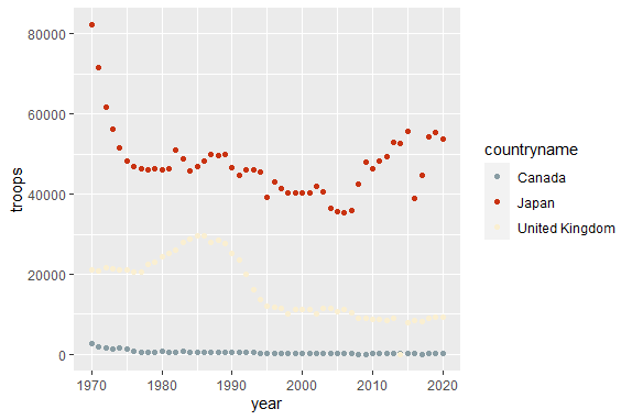
まずは、アメリカ兵のイギリス、日本、カナダへの駐留数の変化を見てみます。

library(troopdata)
library(ggplot2)
library(tidyverse)
library(wesanderson)

hostlist <- c("JPN", "GBR", "CAN")

US_troops <- get_troopdata(host = hostlist, startyear = 1970, endyear = 2020)


US_troops %>% 
  ggplot()+
  geom_point(aes(year, troops, col=countryname))+
  scale_color_manual(values = wes_palette("Royal1"))
  

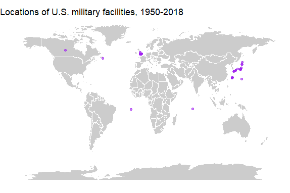
次に、同じ地域でアメリカ軍基地がある場所を見てみます。

US_base <- get_basedata(host = hostlist, country_count = FALSE)
head(US_base)

> head(US_base)
# A tibble: 6 x 9
  countryname   ccode iso3c basename     lat    lon  base lilypad
  <chr>         <dbl> <chr> <chr>      <dbl>  <dbl> <dbl>   <dbl>
1 Ascension Is~   200 GBR   Ascension~ -7.95  -14.4     1       0
2 BR Indian Oc~   200 GBR   Diego Gar~ -7.32   72.4     1       0
3 Canada           20 CAN   NA         56.1  -106.      0       1
4 Canada           20 CAN   Argentia,~ 47.3   -54.0     1       0
5 Japan           740 JPN   Yokota AB~ 35.7   140.      1       0
6 Japan           740 JPN   US Fleet ~ 33.2   130.      1       0
# ... with 1 more variable: fundedsite <dbl>

地図にプロットしてみます。

map <- map_data("world")

basemap <- ggplot() +
  geom_polygon(data = map, aes(x = long, y = lat, group = group), fill = "gray80", color = "white", size = 0.1) +
  geom_point(data = US_base, aes(x = lon, y = lat), color = "purple", alpha = 0.6) +
  coord_equal(ratio = 1.3) +
  theme_void() +
  labs(title = "Locations of US military base in GBR, JPN and CAN, 1950-2018")

4. さいごに

あまり使うことはなさそうですが、何かの時に。