【R】ggside

1. はじめに

ggsideは、ggplotの助けを借りて再度プロットを描画するパッケージです。

2. インストール

Githubからインストールします。

devtools::install_github("jtlandis/ggside")

3. つかってみる

今のところ、以下のgeomが対応しているようです。

• GeomBar
• GeomBoxplot
• GeomDensity
• GeomFreqpoly
• GeomHistogram
• GeomLine
• GeomPath
• GeomPoint
• GeomText
• GeomTile
• GeomViolin

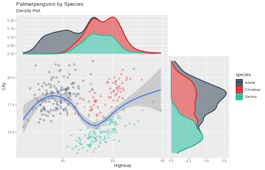
早速使ってみます。この例では、上(y)と右(x)の両方に再度プロットしています。

データはペンギンを使います。

library(ggside)
library(tidyverse)
library(tidyquant)
library(palmerpenguins)

data(penguins)

p2<-penguins %>%
  drop_na() %>% 
  ggplot(aes(bill_length_mm, bill_depth_mm, color = species)) +
  geom_point(size = 2, alpha = 0.3) +
  geom_smooth(aes(color = NULL), se=TRUE) +
  geom_xsidedensity(
    aes(
      y    = after_stat(density),
      fill = species
    ),
    alpha    = 0.5,
    size     = 1,
    position = "stack"
  ) +
  geom_ysidedensity(
    aes(
      x    = after_stat(density),
      fill = species
    ),
    alpha    = 0.5,
    size     = 1,
    position = "stack"
  ) +
  scale_color_tq() +
  scale_fill_tq() +
  theme_tq() +
  labs(title = "Palmerpenguins by Species" ,
       subtitle = "Density Plot",
       x = "Bill Length mm", y = "Bill Depth mm") +  theme(
         ggside.panel.scale.x = 0.4,
         ggside.panel.scale.y = 0.4
       )
plot(p2)

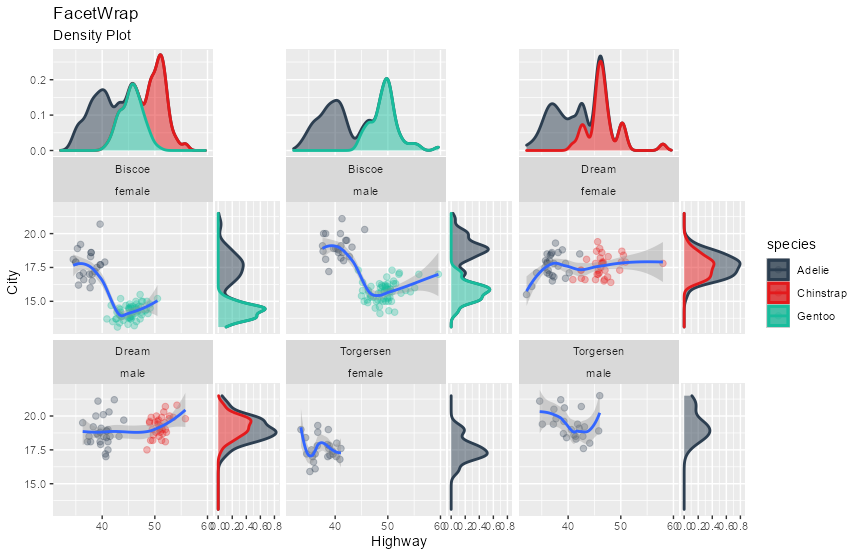
Facetもできます。

p2 + facet_wrap(island~sex) +
  labs(title = "FacetWrap") +
  ggside(collapse = "x")

4. さいごに

サイドプロットは、特長をさらに可視化してくれるので、重宝しますね。