【R】biscale

1. はじめに

biscaleは、2変数をプロットするときに便利なパッケージです。

2. インストール

CRANからインストールできます。

install.packages("biscale")

3. つかってみる

例にあるものを、ほぼそのまま実行してみます。

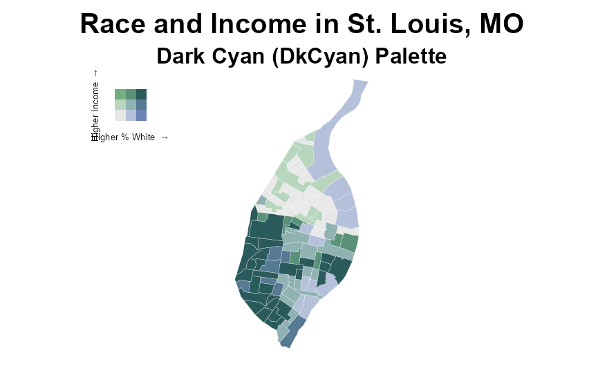
データは、セントルイスの人種と収入に関するデータです。

library(biscale)
library(ggplot2)
library(cowplot)
library(sf)


data <- bi_class(stl_race_income, x = pctWhite, y = medInc, style = "quantile", dim = 3)

> data
Simple feature collection with 106 features and 4 fields
Geometry type: POLYGON
Dimension:     XY
Bounding box:  xmin: -90.32052 ymin: 38.53185 xmax: -90.16657 ymax: 38.77443
Geodetic CRS:  NAD83
First 10 features:
         GEOID  pctWhite medInc bi_class                       geometry
1  29510112100 66.470727  56118      3-3 POLYGON ((-90.30445 38.6328...
2  29510116500 47.799564  43913      2-2 POLYGON ((-90.24302 38.5975...
3  29510110300  2.427686  17448      1-1 POLYGON ((-90.24032 38.6643...
4  29510103700 90.773067  50565      3-3 POLYGON ((-90.29877 38.6028...
5  29510103800 87.733402  74425      3-3 POLYGON ((-90.32052 38.5941...
6  29510104500 74.723618  54286      3-3 POLYGON ((-90.29432 38.6209...
7  29510106100  1.752464  18895      1-1 POLYGON ((-90.29005 38.6705...
8  29510105500  2.376729  36130      1-2 POLYGON ((-90.28601 38.6589...
9  29510105200 36.833277  60938      2-3 POLYGON ((-90.29481 38.6473...
10 29510105300 10.336195  23274      1-1 POLYGON ((-90.29705 38.6617...

プロットしてみます。

map <- ggplot() +
  geom_sf(data = data, mapping = aes(fill = bi_class), color = "white", size = 0.1, show.legend = FALSE) +
  bi_scale_fill(pal = "DkCyan", dim = 3) +
  labs(
    title = "Race and Income in St. Louis, MO",
    subtitle = "Dark Cyan (DkCyan) Palette"
  ) +
  bi_theme()

legend <- bi_legend(pal = "DkCyan",
                    dim = 3,
                    xlab = "Higher % White ",
                    ylab = "Higher Income ",
                    size = 10)


finalPlot <- ggdraw() +
  draw_plot(map, 0, 0, 1, 1) +
  draw_plot(legend, 0.1, .6, 0.2, 0.2)

finalPlot

4. さいごに

地図での表現の幅が広がります。