【R】2標本のｔ検定

架空の話として。。。
都市Aと都市BでPM2.5（微小粒子状物質）の1日の平均観測量を比べた時に、両都市でPM2.5の飛散量に差があるかどうかを以下の手順で検証します。

①架空のデータを作ります。
②ヒストグラムでデータを確認します。
③シャピロ・ウィルクの検定で正規性を確認します。
④分散性を確認します。
⑤ｔ検定します。
⑥2つのヒストグラムを重ねて表示します。
⑦2つのデータを密度プロットしてみます。
⑧バイオリンプロットとボックスプロットでも表示してみます。

#データ生成・・・①
city_a <- rnorm(n=200, mean=20, sd=5.1) #正規分布の架空データ　都市AのPM2.5飛散量
city_b <- rnorm(n=200, mean=25.3, sd=5.4) #正規分布の架空データ　都市BのPM2.5飛散量

#ヒストグラムで確認・・・②
layout(matrix(1:2, 1, 2))
hist(city_a, breaks=seq(0,50,2.5), xlab="range", xlim=c(0,50), ylim=c(0,50))
hist(city_b, breaks=seq(0,50,2.5), xlab="range", xlim=c(0,50), ylim=c(0,50))

何となく正規分布してそうですが、検定にて確認します。

# 正規性の検定・・・③
shapiro.test(city_a)  
shapiro.test(city_b)

> shapiro.test(city_a)  

	Shapiro-Wilk normality test

data:  city_a
W = 0.99264, p-value = 0.4147

> shapiro.test(city_b)

	Shapiro-Wilk normality test

data:  city_b
W = 0.99426, p-value = 0.6389

帰無仮説は棄却されませんので、帰無仮説（正規分布でないとはいえない）を採択して、データは正規分布であるとします。次に、2標本の母分散が等しいかどうかを確認します。

#分散性の検定・・・④
var.test(city_a, city_b)

結果を見ますと、帰無仮説（分散は等しい）が棄却されなかったので、分散はひとしいとします。

> var.test(city_a, city_b)

	F test to compare two variances

data:  city_a and city_b
F = 1.0263, num df = 199, denom df = 199, p-value = 0.8548
alternative hypothesis: true ratio of variances is not equal to 1
95 percent confidence interval:
 0.7767039 1.3561528
sample estimates:
ratio of variances 
          1.026318 

分散が等しいとして、ｔ検定をします。

#t 検定・・・⑤
t.test(city_a, city_b, var.equal = T)

	Two Sample t-test

data:  city_a and city_b
t = -8.3495, df = 398, p-value = 1.147e-15
alternative hypothesis: true difference in means is not equal to 0
95 percent confidence interval:
 -5.671072 -3.509467
sample estimates:
mean of x mean of y 
 20.05004  24.64030 

この結果、2つの都市で差があるといえます。

続いて、2標本をいろいろなプロットで表示してみます。

dat_a<-data.frame("City"=c(rep("city_a", length(city_a))), "Val"=city_a)
dat_b<-data.frame("City"=c(rep("city_b", length(city_b))), "Val"=city_b)
dat<-rbind(dat_a, dat_b)

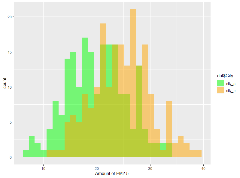
# 2つのヒストグラムをまとめて表示・・・⑥
library(ggplot2)
ggplot(dat) + #データフレーム指定
  geom_histogram(aes(x=dat$Val, fill=dat$City),  #描画対象の変数
                 position="identity", #重ねて描画
                 alpha=0.5,
                 bandwidth=2) +
  scale_fill_manual(values=c("green", "orange")) +
  labs(x="Amount of PM2.5")
  
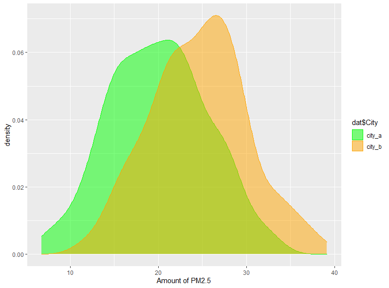
# 都市で色分けして密度プロットを描く・・・⑦
ggplot(dat) + #データフレーム指定
  geom_density(aes(x=dat$Val, 
                   color=dat$City,
                   fill=dat$City),
                   alpha=0.5) +
  scale_color_manual(values=c("green", "orange"))+
  scale_fill_manual(values=c("green", "orange"))+
  labs(x="Amount of PM2.5")

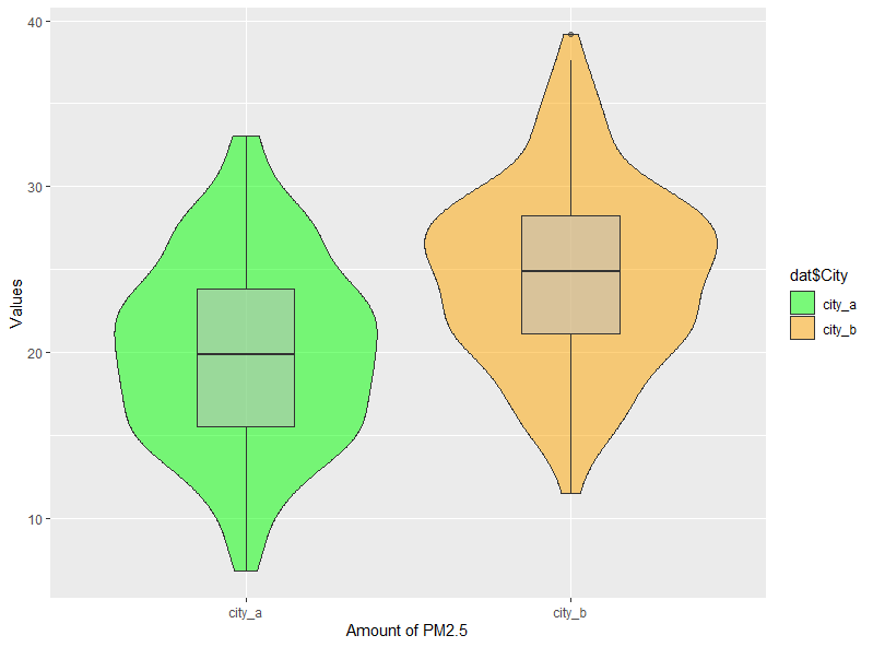
# バイオリンプロットとボックスプロットを重ねて描く・・・⑧
ggplot(dat) + #データフレーム指定
  geom_violin(aes(y   =dat$Val, 
                  x   =dat$City, 
                  fill=dat$City),
                  alpha=0.5) +
  geom_boxplot(aes(y   =dat$Val, 
                   x   =dat$City), 
                   fill="grey",
                   width=0.3,
                   alpha=0.5) +
  scale_color_manual(values=c("green", "orange"))+
  scale_fill_manual(values=c("green", "orange"))+
  labs(x="Amount of PM2.5", y="Values")