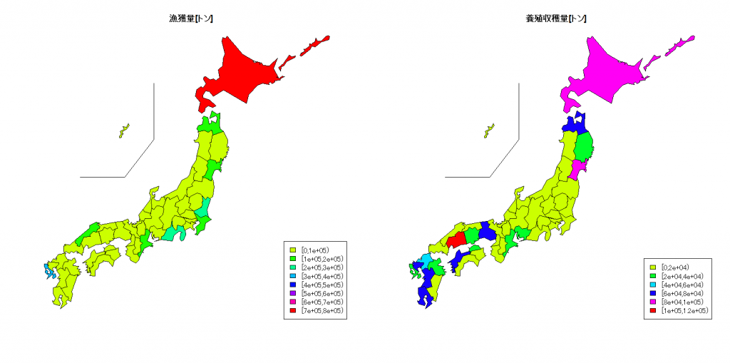
総務省統計局が発表している「都道府県・市区町村のすがた(社会・人口統計体系)」から、都道府県別の漁獲量[トン]と養殖収穫量[トン]を表示します。2017年のデータです。
| 都道府県 |
漁獲量 |
養殖収穫量 |
| 北海道 |
746592 |
82596 |
| 青森 |
107331 |
79585 |
| 岩手 |
76509 |
37817 |
| 宮城 |
158734 |
91635 |
| 秋田 |
6198 |
269 |
| 山形 |
4712 |
229 |
| 福島 |
52876 |
1311 |
| 茨城 |
297896 |
0 |
| 栃木 |
277 |
763 |
| 群馬 |
3 |
376 |
| 埼玉 |
1 |
2 |
| 千葉 |
120150 |
8636 |
| 東京 |
40939 |
0 |
| 神奈川 |
32804 |
1231 |
| 新潟 |
30602 |
1407 |
| 富山 |
23837 |
84 |
| 石川 |
37486 |
1941 |
| 福井 |
0 |
272 |
| 山梨 |
0 |
994 |
| 長野 |
158 |
1607 |
| 岐阜 |
264 |
1413 |
| 静岡 |
202229 |
5862 |
| 愛知 |
70005 |
20892 |
| 三重 |
154852 |
26276 |
|
| 都道府県 |
漁獲量 |
養殖収穫量 |
| 滋賀 |
0 |
598 |
| 京都 |
8688 |
680 |
| 大阪 |
19291 |
0 |
| 兵庫 |
41053 |
71119 |
| 奈良 |
0 |
21 |
| 和歌山 |
18808 |
3706 |
| 鳥取 |
74316 |
1830 |
| 島根 |
136948 |
523 |
| 岡山 |
3906 |
21637 |
| 広島 |
16127 |
107312 |
| 山口 |
25804 |
2567 |
| 徳島 |
10701 |
11686 |
| 香川 |
16373 |
25479 |
| 愛媛 |
79867 |
62827 |
| 高知 |
65751 |
18878 |
| 福岡 |
25692 |
50044 |
| 佐賀 |
8053 |
68585 |
| 長崎 |
317069 |
23109 |
| 熊本 |
18009 |
62539 |
| 大分 |
31945 |
23098 |
| 宮崎 |
96582 |
17239 |
| 鹿児島 |
0 |
61624 |
| 沖縄 |
15954 |
0 |
|
|
library(leaflet)
library(knitr)
library(kableExtra)
library(dplyr)
library(tidyr)
library(stringr)

dat <- read.csv("http://www.dinov.tokyo/Data/JP_Pref/Pref_data.csv", header = TRUE, fileEncoding="UTF-8")
col_start <- 0.2
col_end <- 0.0

table_df<-data.frame(都道府県=dat$都道府県, 漁獲量=dat$漁獲量, 養殖収穫量=dat$養殖収穫量)

datc_k <- cut(dat$漁獲量, hist(dat$漁獲量, plot=FALSE)$breaks, right=FALSE)
datc_kcol <- rainbow(length(levels(datc_k)), start = col_start, end=col_end)[as.integer(datc_k)]
datc_m <- cut(dat$養殖収穫量, hist(dat$養殖収穫量, plot=FALSE)$breaks, right=FALSE)
datc_mcol <- rainbow(length(levels(datc_m)), start = col_start, end=col_end)[as.integer(datc_m)]
windowsFonts(JP4=windowsFont("Biz Gothic"))
windows(width=1600, height=800)
par(family="JP4")
layout(matrix(1:2, 1, 2))

library(NipponMap)
JapanPrefMap(datc_kcol, main="漁獲量[トン]")
legend("bottomright", fill=rainbow(length(levels(datc_k)), start = col_start, end=col_end), legend=names(table(datc_k)))
JapanPrefMap(datc_mcol, main="養殖収穫量[トン]")
legend("bottomright", fill=rainbow(length(levels(datc_m)), start = col_start, end=col_end), legend=names(table(datc_m)))

library(clipr)
t1=kable(table_df[c(1:24),], align = "c", row.names=FALSE) %>%
  kable_styling(full_width = F) %>%
  column_spec(1, bold = T) %>%
  collapse_rows(columns = 1, valign = "middle")
t2=kable(table_df[c(25:47),], align = "c", row.names=FALSE) %>%
  kable_styling(full_width = F) %>%
  column_spec(1, bold = T) %>%
  collapse_rows(columns = 1, valign = "middle")
paste(c('<table><tr valign="top"><td>', t1, '</td><td>', t2, '</td><tr></table>'), sep = '') %>% write_clip

