【R】因子分析とクラスタリング

１．はじめに

こちらでは、mtcarsのデータを用いて因子分析をしました。今回は、この後にクラスタリングまで行ってみたいと思います。

２．因子分析

２．１　因子数を決める

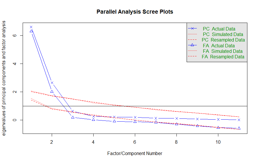
psychパッケージの並行分析の関数fa.parallelを用いてスクリープロットをひょじします。この結果、1以上である因子数を２とします。

library(psych)

#スクリープロットで因子数を決める。
result.prl<-fa.parallel(mtcars, fm="ml")

２．２　因子分析

因子分析をし、結果を表示します。

#因子分析
retFA<-fa(mtcars, nfactors=2, fm="ml", rotate="carimax", sores="regression")

#結果を表示
print(retFA, digits=2, sort=TRUE)

Factor Analysis using method =  ml
Call: fa(r = mtcars, nfactors = 2, rotate = "carimax", fm = "ml", 
    sores = "regression")
Standardized loadings (pattern matrix) based upon correlation matrix
     item   ML1   ML2   h2    u2 com
cyl     2  0.96  0.06 0.93 0.070 1.0
disp    3  0.95 -0.09 0.90 0.096 1.0
mpg     1 -0.91  0.07 0.83 0.167 1.0
wt      6  0.87 -0.28 0.83 0.168 1.2
hp      4  0.85  0.36 0.86 0.143 1.4
vs      8 -0.78 -0.36 0.74 0.256 1.4
drat    5 -0.73  0.42 0.70 0.298 1.6
qsec    7 -0.53 -0.75 0.85 0.150 1.8
am      9 -0.58  0.70 0.83 0.171 1.9
gear   10 -0.51  0.70 0.75 0.246 1.8
carb   11  0.54  0.57 0.61 0.386 2.0

                       ML1  ML2
SS loadings           6.44 2.41
Proportion Var        0.59 0.22
Cumulative Var        0.59 0.80
Proportion Explained  0.73 0.27
Cumulative Proportion 0.73 1.00

Mean item complexity =  1.5
Test of the hypothesis that 2 factors are sufficient.

The degrees of freedom for the null model are  55  and the objective function was  15.4 with Chi Square of  408.01
The degrees of freedom for the model are 34  and the objective function was  2.72 

The root mean square of the residuals (RMSR) is  0.05 
The df corrected root mean square of the residuals is  0.06 

The harmonic number of observations is  32 with the empirical chi square  7.66  with prob <  1 
The total number of observations was  32  with Likelihood Chi Square =  68.57  with prob <  4e-04 

Tucker Lewis Index of factoring reliability =  0.832
RMSEA index =  0.175  and the 90 % confidence intervals are  0.118 0.243
BIC =  -49.27
Fit based upon off diagonal values = 0.99
Measures of factor score adequacy             
                                                   ML1  ML2
Correlation of (regression) scores with factors   0.99 0.96
Multiple R square of scores with factors          0.98 0.92
Minimum correlation of possible factor scores     0.96 0.85

因子ML1>ML2の組（cyl, disp, mpg, wt, hp, vs, drat）とML1<ML2の組（qsec, am ,gear, carb）に分けられそうです。

２．３　ダイアグラム

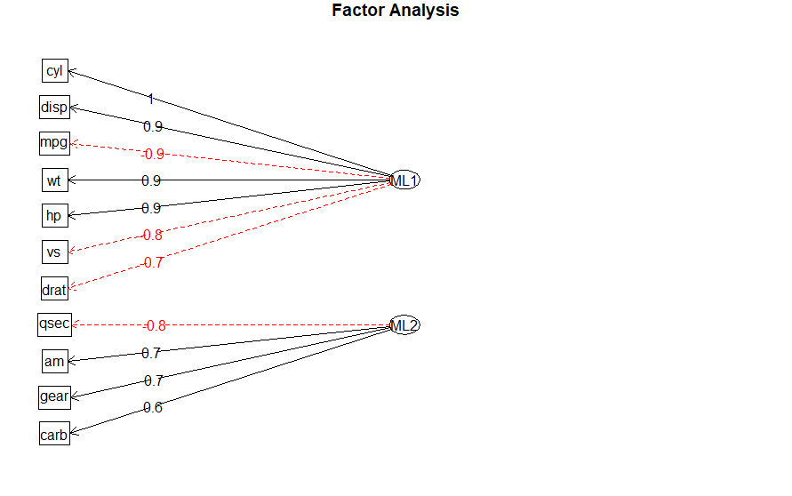
因子分析の結果をダイアグラムで表示してみます。

#ダイアグラムで表示
fa.diagram(retFA)

２．４　散布図

因子１と因子２の関係を散布図で表してみます。

#因子１と因子２の関係をプロットしてみる
plot(retFA$loadings[,1], retFA$loadings[,2], type="n")
text(retFA$loadings[,1], retFA$loadings[,2], rownames(retFA$loadings), col="steelblue")
lines(c(-1,1), c(0,0), col="grey")
lines(c(0,0), c(-1,1), col="grey")

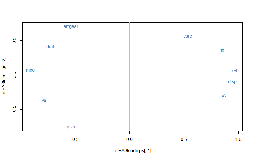
因子の解釈が難しいですが、仮に因子１をスペック(spec)に関するもの、因子２を快適さ(comfort)に関するものとします。

３．クラスタリング

クラスタリングの手法はいろいろありますが、ここではk-平均法(kmeans())を使います。実行結果は、実行のたびに異なるらしいです。

#k-平均法でクラスタリング
dfFA<-as.data.frame(retFA$scores)
rownames(dfFA)<-rownames(mtcars)
colnames(dfFA)<-c("spec", "comfort")

#クラスタリングを可視化
kmFA<-kmeans(dfFA, 3, iter.max=50)
color.kmFA<-kmFA$cluster
color.kmFA<-as.character(color.kmFA)
levels(color.kmFA)<-c("blue", "red", "green")
head(color.kmFA)
color.kmFA<-as.character(color.kmFA)
plot(dfFA$spec, dfFA$comfort, type="n")
text(dfFA$spec, dfFA$comfort, rownames(dfFA), col=color.kmFA)
lines(c(-1,1), c(0,0), col="grey")
lines(c(0,0), c(-1,1), col="grey")

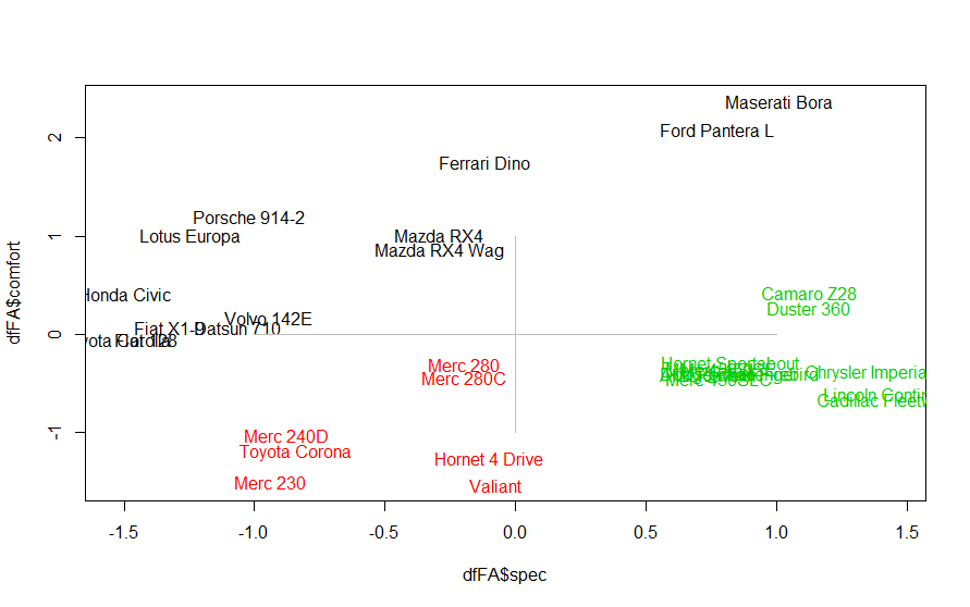
どう解釈してよいかわかりませんが、練習ということで。。。