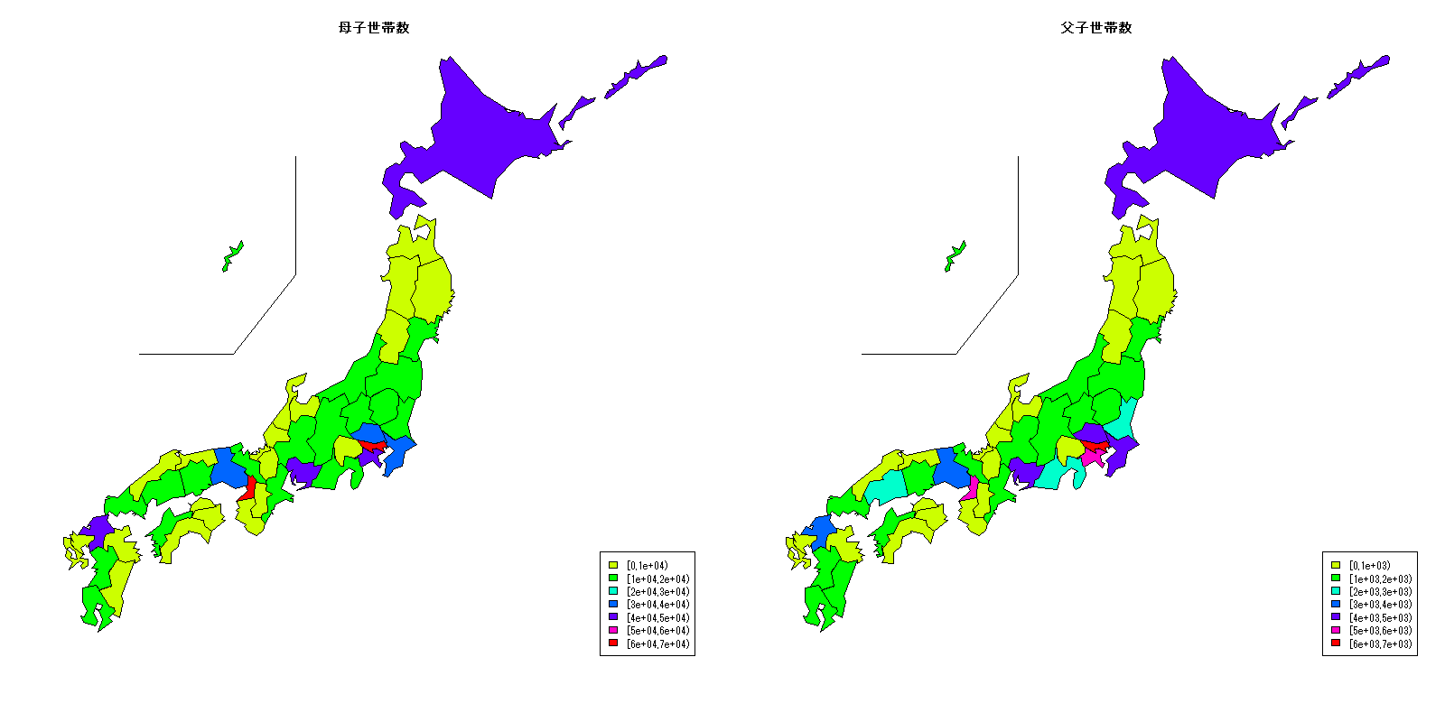
総務省統計局が発表している「都道府県・市区町村のすがた(社会・人口統計体系)」から、都道府県別の母子家庭、父子家計の世帯数を示してみたいと思います。2015年のデータです。

| 都道府県 |
母子世帯数 |
父子世帯数 |
| 北海道 |
45651 |
4481 |
| 青森 |
9415 |
973 |
| 岩手 |
7126 |
828 |
| 宮城 |
12767 |
1327 |
| 秋田 |
4781 |
517 |
| 山形 |
5265 |
547 |
| 福島 |
10792 |
1246 |
| 茨城 |
16215 |
2146 |
| 栃木 |
10708 |
1379 |
| 群馬 |
11811 |
1482 |
| 埼玉 |
35849 |
4917 |
| 千葉 |
30074 |
4288 |
| 東京 |
60848 |
6211 |
| 神奈川 |
44040 |
5680 |
| 新潟 |
10538 |
1142 |
| 富山 |
4613 |
616 |
| 石川 |
5661 |
721 |
| 福井 |
3572 |
415 |
| 山梨 |
5070 |
630 |
| 長野 |
10997 |
1320 |
| 岐阜 |
10327 |
1173 |
| 静岡 |
19730 |
2445 |
| 愛知 |
40919 |
4852 |
| 三重 |
10195 |
1349 |
|
| 都道府県 |
母子世帯数 |
父子世帯数 |
| 滋賀 |
7225 |
884 |
| 京都 |
16581 |
1575 |
| 大阪 |
64842 |
5914 |
| 兵庫 |
33927 |
3515 |
| 奈良 |
8270 |
748 |
| 和歌山 |
7544 |
780 |
| 鳥取 |
3700 |
362 |
| 島根 |
3714 |
411 |
| 岡山 |
11561 |
1326 |
| 広島 |
18997 |
2125 |
| 山口 |
10158 |
1039 |
| 徳島 |
4614 |
556 |
| 香川 |
6396 |
750 |
| 愛媛 |
10060 |
1141 |
| 高知 |
5986 |
728 |
| 福岡 |
40071 |
3646 |
| 佐賀 |
5518 |
521 |
| 長崎 |
9930 |
959 |
| 熊本 |
12785 |
1181 |
| 大分 |
7778 |
760 |
| 宮崎 |
9918 |
1018 |
| 鹿児島 |
13746 |
1641 |
| 沖縄 |
14439 |
1738 |
|
|
library(leaflet)
library(knitr)
library(kableExtra)
library(dplyr)
library(tidyr)
library(stringr)

dat <- read.csv("http://www.dinov.tokyo/Data/JP_Pref/Pref_data.csv", header = TRUE, fileEncoding="UTF-8")
col_start <- 0.2
col_end <- 0.0

table_df<-data.frame(都道府県=dat$都道府県, 母子世帯数=dat$母子世帯数, 父子世帯数=dat$父子世帯数)

datc_k <- cut(dat$母子世帯数, hist(dat$母子世帯数, plot=FALSE)$breaks, right=FALSE)
datc_kcol <- rainbow(length(levels(datc_k)), start = col_start, end=col_end)[as.integer(datc_k)]
datc_m <- cut(dat$父子世帯数, hist(dat$父子世帯数, plot=FALSE)$breaks, right=FALSE)
datc_mcol <- rainbow(length(levels(datc_m)), start = col_start, end=col_end)[as.integer(datc_m)]

library(NipponMap)
windowsFonts(JP4=windowsFont("Biz Gothic"))
windows(width=1600, height=800)

png("0plot1.png", width = 1600, height = 800)
par(family="JP4")
layout(matrix(1:2, 1, 2))
JapanPrefMap(datc_kcol, main="母子世帯数")
legend("bottomright", fill=rainbow(length(levels(datc_k)), start = col_start, end=col_end), legend=names(table(datc_k)))
JapanPrefMap(datc_mcol, main="父子世帯数")
legend("bottomright", fill=rainbow(length(levels(datc_m)), start = col_start, end=col_end), legend=names(table(datc_m)))
dev.off()

library(clipr)
t1=kable(table_df[c(1:24),], align = "c", row.names=FALSE) %>%
  kable_styling(full_width = F) %>%
  column_spec(1, bold = T) %>%
  collapse_rows(columns = 1, valign = "middle")
t2=kable(table_df[c(25:47),], align = "c", row.names=FALSE) %>%
  kable_styling(full_width = F) %>%
  column_spec(1, bold = T) %>%
  collapse_rows(columns = 1, valign = "middle")
paste(c('<table><tr valign="top"><td>', t1, '</td><td>', t2, '</td><tr></table>'), sep = '') %>% write_clip