【R】tidymodels の Tuning
1. はじめに
機械学習でどのようにパラメータのチューニングをすればよいかのお勉強。TidymodelsのページとJulia Silge氏のYouTube「Tuning random forest hyperparameters with tidymodels」と「Hyperparameter tuning using tidymodels」を参考にしました。
Swiss Bank Note のパラメータ=6か所の長さの測定結果から、ニセ札かどうかを分類する機械学習を行います。
2. データ
使用するデータは、Wolfram Data RepositoryからSwiss Bank Noteというデータを用います。これは、1988年に、B. Flury and H. Riedwylが発表したデータで、100のニセ札と100の本物のお札について、お札の6か所の長さを測ったものです。
上記のWolfram Data RepositoryのデータをCSV形式でダウンロードしましたが、そのままでは使いにくいので、少し修正しました。
# libraries ---------------------------------------------------------------
library(tidyverse)
library(tidymodels)
# data --------------------------------------------------------------------
banknote_df <- read.csv("http://www.dinov.tokyo/Data/JP_Pref/Sample-Data-Swiss-Bank-Notes.csv")
head(banknote_df)
  Length  Left Right Bottom  Top Diagonal Genuine.Counterfeit
1  214.8 131.0 131.1    9.0  9.7    141.0         counterfeit
2  214.6 129.7 129.7    8.1  9.5    141.7         counterfeit
3  214.8 129.7 129.7    8.7  9.6    142.2         counterfeit
4  214.8 129.7 129.6    7.5 10.4    142.0         counterfeit
5  215.0 129.6 129.7   10.4  7.7    141.8         counterfeit
6  215.7 130.8 130.5    9.0 10.1    141.4         counterfeit
3. 機械学習
3.1 データ準備
トレーニングデータとテストデータを準備します。元のデータを3:1に分割します。
# 1: Initial Split --------------------------------------------------------
set.seed(1234)

banknote_split <- initial_split(banknote_df, strada = Genuine.Counterfeit)

banknote_train <- training(banknote_split)
head(banknote_train)
banknote_test <- testing(banknote_split)
head(banknote_test)
> banknote_train <- training(banknote_split)
> head(banknote_train)
  Length  Left Right Bottom  Top Diagonal Genuine.Counterfeit
1  214.8 131.0 131.1    9.0  9.7    141.0         counterfeit
2  214.6 129.7 129.7    8.1  9.5    141.7         counterfeit
3  214.8 129.7 129.7    8.7  9.6    142.2         counterfeit
4  214.8 129.7 129.6    7.5 10.4    142.0         counterfeit
5  215.0 129.6 129.7   10.4  7.7    141.8         counterfeit
6  215.7 130.8 130.5    9.0 10.1    141.4         counterfeit
> banknote_test <- testing(banknote_split)
> head(banknote_test)
   Length  Left Right Bottom  Top Diagonal Genuine.Counterfeit
8   214.5 129.6 129.2    7.2 10.7    141.7         counterfeit
10  215.2 130.4 130.3    9.2 10.0    140.7         counterfeit
17  214.6 129.9 130.1    8.2  9.8    141.7         counterfeit
19  215.2 129.6 129.6    7.4 11.5    141.5         counterfeit
20  214.7 130.2 129.9    8.6 10.0    141.9         counterfeit
22  215.6 130.5 130.0    8.1 10.3    141.6         counterfeit
3.2 レシピ
目的変数を”Genuine.Counterfeit”として、レシピを準備します。
# 2: Preprocessing --------------------------------------------------------

banknote_rec <- recipe(Genuine.Counterfeit ~ ., data = banknote_train)

banknote_prep <- prep(banknote_rec)
juiced <- juice(banknote_prep)
> juiced
# A tibble: 150 x 7
   Length  Left Right Bottom   Top Diagonal Genuine.Counterfeit
    <dbl> <dbl> <dbl>  <dbl> <dbl>    <dbl> <fct>
 1   215.  131   131.    9     9.7     141  counterfeit
 2   215.  130.  130.    8.1   9.5     142. counterfeit
 3   215.  130.  130.    8.7   9.6     142. counterfeit
 4   215   130.  130.   10.4   7.7     142. counterfeit
 5   216.  131.  130.    9    10.1     141. counterfeit
 6   216.  130.  130.    7.9   9.6     142. counterfeit
 7   214.  130.  129.    7.2  10.7     142. counterfeit
 8   215.  129.  130.    8.2  11       142. counterfeit
 9   215.  130.  130.    9.2  10       141. counterfeit
10   215.  130.  130.    7.9  11.7     142. counterfeit
# ... with 140 more rows
3.3 モデルとチューニングの仕様
モデルとチューニングの仕様を決めます。ランダムフォレストを使用し、modelは分類、エンジンはrangerとします。mtryとmin_nをチューニングします。
# 3, 4: Model Specification & Hyperparameter Tuning Specification --------------------------------------------------
banknote_spec <- rand_forest(
  mtry = tune(),
  trees = 1000,
  min_n = tune()
) %>%
  set_mode("classification") %>%
  set_engine("ranger")
> banknote_spec
Random Forest Model Specification (classification)

Main Arguments:
  mtry = tune()
  trees = 1000
  min_n = tune()

Computational engine: ranger
3.4 ワークフロー
これらをまとめて、ワークフローに定義します。
# 5: Bundle into Workflow -------------------------------------------------

tune_wf <- workflow() %>%
  add_recipe(banknote_rec) %>%
  add_model(banknote_spec)
> tune_wf
== Workflow ====================================================================
Preprocessor: Recipe
Model: rand_forest()

-- Preprocessor ----------------------------------------------------------------
0 Recipe Steps

-- Model -----------------------------------------------------------------------
Random Forest Model Specification (classification)

Main Arguments:
  mtry = tune()
  trees = 1000
  min_n = tune()

Computational engine: ranger
3.5 クロスバリデーション準備
# 6: Cross Validation -----------------------------------------------------
set.seed(234)
banknote_fold <- vfold_cv(banknote_train)
> banknote_fold
#  10-fold cross-validation
# A tibble: 10 x 2
   splits           id
   <named list>     <chr>
 1 <split [135/15]> Fold01
 2 <split [135/15]> Fold02
 3 <split [135/15]> Fold03
 4 <split [135/15]> Fold04
 5 <split [135/15]> Fold05
 6 <split [135/15]> Fold06
 7 <split [135/15]> Fold07
 8 <split [135/15]> Fold08
 9 <split [135/15]> Fold09
10 <split [135/15]> Fold10
3.6 チューニング
20個のグリッドに分け、チューニングしてみます。
# 7: Tune -----------------------------------------------------------------
doParallel::registerDoParallel()
set.seed(345)
tune_res <- tune_grid(
  tune_wf,
  resamples = banknote_fold,
  grid = 20
)
結果を見ますと。
> tune_res %>%
+ collect_metrics()
# A tibble: 40 x 7
mtry min_n .metric .estimator mean n std_err
<int> <int> <chr> <chr> <dbl> <int> <dbl>
1 1 6 accuracy binary 0.993 10 0.00667
2 1 6 roc_auc binary 1 10 0
3 1 39 accuracy binary 0.993 10 0.00667
4 1 39 roc_auc binary 0.998 10 0.002
5 2 15 accuracy binary 0.993 10 0.00667
6 2 15 roc_auc binary 1 10 0
7 2 17 accuracy binary 0.993 10 0.00667
8 2 17 roc_auc binary 1 10 0
9 2 30 accuracy binary 0.993 10 0.00667
10 2 30 roc_auc binary 1 10 0
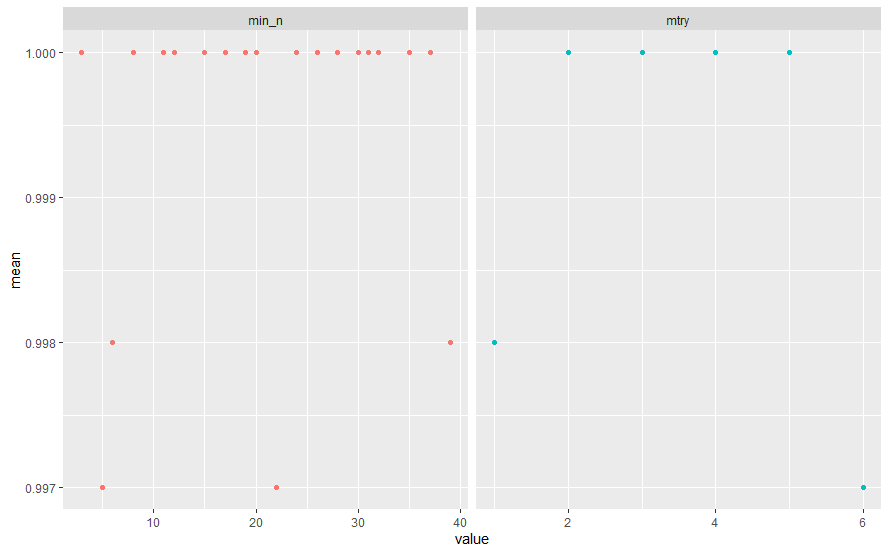
# ... with 30 more rowsこの時点で、これ以上のチューニングは不要では。。。?
tune_res %>%
  collect_metrics() %>%
  filter(.metric == "roc_auc") %>%
  select(mean, min_n, mtry) %>%
  pivot_longer(min_n:mtry,
               values_to = "value",
               names_to = "parameter") %>%
  ggplot(aes(value, mean, color=parameter)) +
  geom_point(show.legend = FALSE) +
  facet_wrap(~ parameter, scales = "free_x")
練習のため、少しパラメータをいじって、再度実施してみます。
rf_grid <- grid_regular(
  mtry(range = c(2, 5)),
  min_n( range = c(10, 20)),
  levels = 5
)
set.seed(456)
regular_res <- tune_grid(
  tune_wf,
  resamples = banknote_fold,
  grid = rf_grid
)
> regular_res %>%
+   collect_metrics()
# A tibble: 40 x 7
    mtry min_n .metric  .estimator  mean     n std_err
   <int> <int> <chr>    <chr>      <dbl> <int>   <dbl>
 1     2    10 accuracy binary     0.987    10 0.00889
 2     2    10 roc_auc  binary     1        10 0
 3     2    12 accuracy binary     0.993    10 0.00667
 4     2    12 roc_auc  binary     1        10 0
 5     2    15 accuracy binary     0.993    10 0.00667
 6     2    15 roc_auc  binary     1        10 0
 7     2    17 accuracy binary     0.993    10 0.00667
 8     2    17 roc_auc  binary     1        10 0
 9     2    20 accuracy binary     0.993    10 0.00667
10     2    20 roc_auc  binary     1        10 0
# ... with 30 more rows
結果は、良くはなりましたが。。。
3.7 ファイナライズ
このモデルで良さそうなので、モデルのファイナライズをします。
# 9: Finalize Workflow ----------------------------------------------------

best_auc <- select_best(regular_res, "roc_auc")

final_rf <- finalize_model(
  banknote_spec,
  best_auc
)


# 10: Final Fit -----------------------------------------------------------

library(vip)

final_rf %>%
  set_engine("ranger", importance = "permutation") %>%
  fit(Genuine.Counterfeit ~ .,
      data = juice(banknote_prep)) %>%
  vip(geom = "point")

final_wf <- workflow() %>%
  add_recipe(banknote_rec) %>%
  add_model(final_rf)

final_res <- final_wf %>%
  last_fit(banknote_split)
3.8 評価
最終的な評価をします。
# 11: Evaluate ------------------------------------------------------------

final_res %>%
  collect_metrics()

final_res %>%
  collect_predictions() %>%
  conf_mat(truth = Genuine.Counterfeit, estimate = .pred_class)
> final_res %>%
+   collect_metrics()
# A tibble: 2 x 3
  .metric  .estimator .estimate
  <chr>    <chr>          <dbl>
1 accuracy binary             1
2 roc_auc  binary             1

> final_res %>%
+   collect_predictions() %>%
+   conf_mat(truth = Genuine.Counterfeit, estimate = .pred_class)
             Truth
Prediction    counterfeit genuine
  counterfeit          25       0
  genuine               0      25
すごいですね。認識率100%!
4.さいごに
今回は、あまりチューニングの意味がなかったとおもいますが、勉強にはなりました。
