【R】cartogram
2020年11月27日
1. はじめに
cartogramは、地図の一つで、その地域のある数値情報の大小によって境界を歪めて表現したものです。例えば、人口が多いとふくらましたり、税収が少ないとしぼめたりします。Rを使って描画してみます。
2. インストール
CRANからインストールできます。
install.packages("cartogram")3. 使ってみる
stDataパッケージにあるニュージーランドのデータnzを使って、ニュージーランドの各州の人口の情報でcartogramを描いてみます。
library(viridis)
library(ggplot2)
library(sf)
library(cartogram)
library(spData)
library(tidyverse)
library(sf)
library(ggrepel)
library(patchwork)

data(nz)

nz_dat <- nz %>%
  mutate(
    centroid = st_centroid(geom),
    x = st_coordinates(centroid)[, 1],
    y = st_coordinates(centroid)[, 2]
  ) %>%
  arrange(desc(Population))

map1 <- nz_dat %>%
  ggplot() +
  geom_sf(aes(fill = Population)) +
  coord_sf(datum = NA) +
  scale_fill_viridis_c(alpha = 0.6) +
  labs( title = "New Zealand Population" )  +
  theme_void()+
  geom_text_repel(aes(x = x, y = y, label = Name), col="black", size = 3)

nz_carto = cartogram_cont(nz_dat, "Population", itermax = 5)

map2 <- nz_carto %>%
  ggplot() +
  geom_sf(aes(fill = Population)) +
  coord_sf(datum = NA) +
  scale_fill_viridis_c(alpha = 0.6) +
  theme_void()+
  geom_text_repel(aes(x = x, y = y, label = Name), col="black", size = 3)

map1 | map2
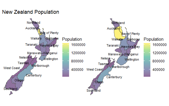
左が通常の境界線で人口毎のコロプレス図を描いたもの、右が人口により境界を変形させたcartogramで描いた地図です。
人口の一覧を表にしてみます。
library(kableExtra)
library(clipr)

table_df<-data.frame(州名=nz_dat$Name, 人口=nz_dat$Population)

table_df %>%
  kable(align = "c", row.names=FALSE) %>%
  kable_styling(full_width = F) %>%
  column_spec(1, bold = T) %>%
  collapse_rows(columns = 1, valign = "middle") %>%
  write_clip
| 州名 | 人口 |
|---|---|
| Auckland | 1657200 |
| Canterbury | 612000 |
| Wellington | 513900 |
| Waikato | 460100 |
| Bay of Plenty | 299900 |
| Manawatu-Wanganui | 234500 |
| Otago | 224200 |
| Northland | 175500 |
| Hawke’s Bay | 164000 |
| Taranaki | 118000 |
| Southland | 98300 |
| Nelson | 51400 |
| Tasman | 51100 |
| Gisborne | 48500 |
| Marlborough | 46200 |
| West Coast | 32400 |
4. 最後に
その地域の情報により境界を変形させると数値の大小が一目瞭然です。が、なんだか変な感じがして、個人的にはイマイチです・・・・。