【R】ggplotify

1. はじめに

ggplotifyは、グラフを柔軟に表示・配置できるようにするためのパッケージです。

2. インストール

CRANからインストールできます。

install.packages("ggplotify")

3. つかってみる

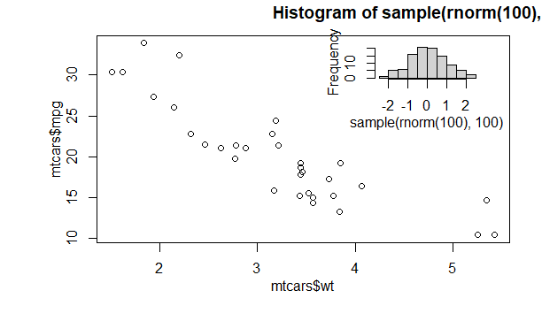
こんな感じ。使いこなすには、gridやgrobの知識も必要そうです。

library("grid")
library("ggplotify")


p1 <- as.grob(~plot(mtcars$wt, mtcars$mpg))
p2 <- as.grob(~hist(sample(rnorm(100), 100)))

grid.newpage()
grid.draw(p1)
vp = viewport(x=.75, y=.75, width=.3, height=.25)
pushViewport(vp)
grid.draw(p2)
upViewport()

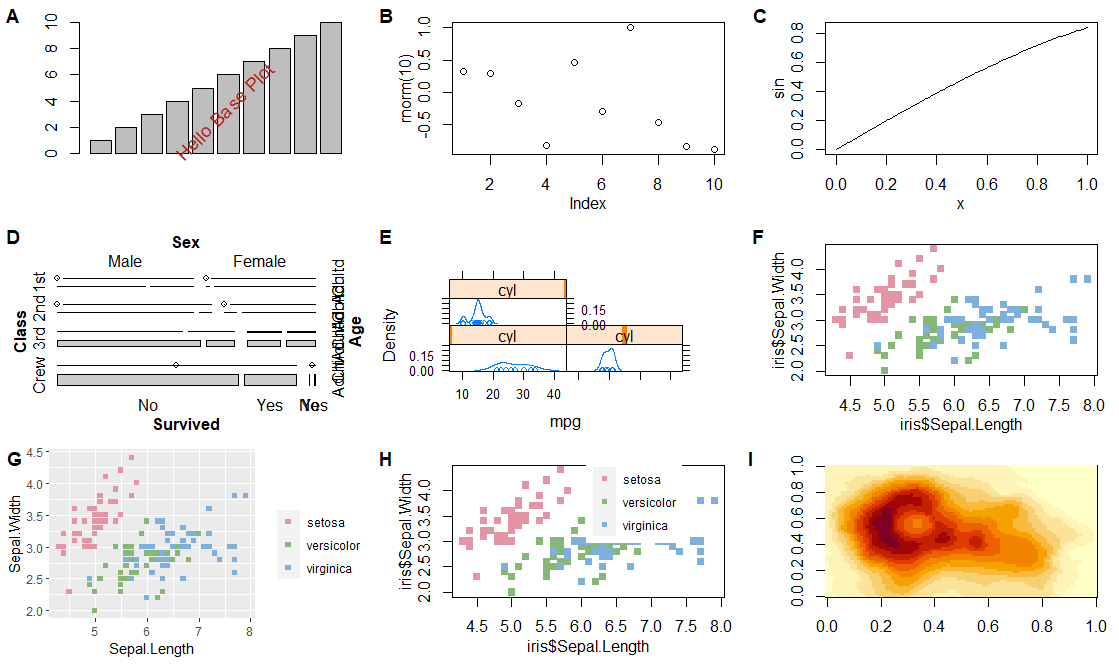
ggplotもサポートしているようです。

library(cowplot)
library(colorspace)
library(grid)
library(vcd)
library(lattice)
library(ggplot2)
p1 <- as.ggplot(~barplot(1:10)) +
  annotate("text", x = .6, y = .5,
           label = "Hello Base Plot", size = 5,
           color = 'firebrick', angle=45)

p2 <- as.ggplot(expression(plot(rnorm(10))))
p3 <- as.ggplot(function() plot(sin))

p4 <- as.ggplot(~mosaic(Titanic))

p5 <- as.ggplot(densityplot(~mpg|cyl, data=mtcars))

col <- rainbow_hcl(3)
names(col) <- unique(iris$Species)

color <- col[iris$Species]
p6 <- as.ggplot(~plot(iris$Sepal.Length, iris$Sepal.Width, col=color, pch=15))

p7 <- ggplot(iris, aes(Sepal.Length, Sepal.Width, color=Species)) +
  geom_point(shape=15) + scale_color_manual(values=col, name="")

legend <- get_legend(p7)

## also able to annotate base or other plots using ggplot2
library(ggimage)
p8 <- p6 + geom_subview(x=.7, y=.78, subview=legend)


p9 <- as.ggplot(~image(volcano))

plot_grid(p1, p2, p3, p4, p5, p6, p7, p8, p9, ncol=3, labels=LETTERS[1:9])

4. さいごに

なかなか大変そうですが、使いこなすと良いパッケージな気がします。