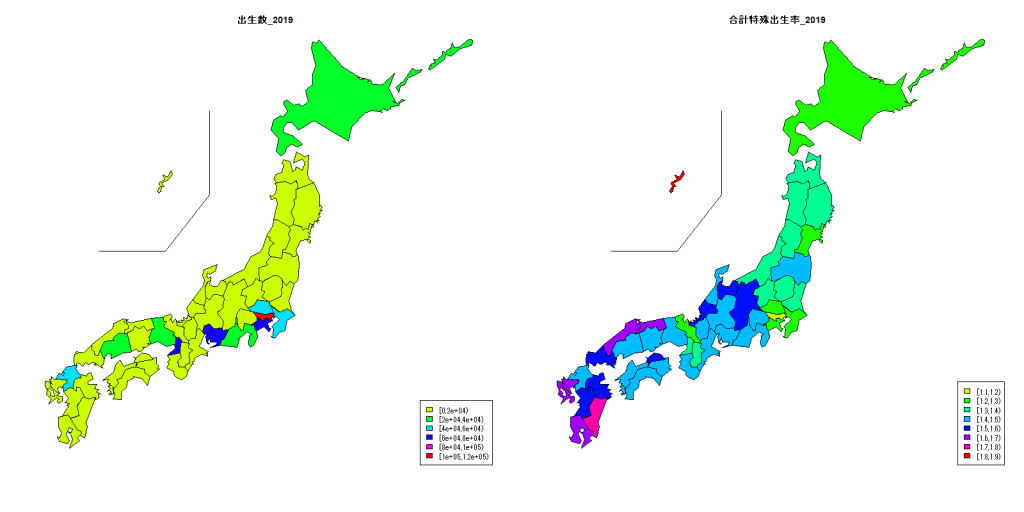
厚生労働省が、6月5日に令和元年(2019)人口動態統計月報年計(概数)の概況を発表しました。少子高齢化社会として心配なのは、やはり出生率です。この統計では、1人の女性が生涯に生む子どもの数にあたる合計特殊出生率も公表され、1.36と前年より0.06ポイント下がりました。これは、4年連続の低下で2007年以来12年ぶりの低水準だそうです。このページにある統計表(xlsファイル)から、都道府県別の出生数と合計特殊出生率を示してみます。
| 都道府県 |
出生数_2019 |
合計特殊出生率_2019 |
| 北海道 |
32642 |
1.24 |
| 青森 |
7803 |
1.38 |
| 岩手 |
7615 |
1.35 |
| 宮城 |
16211 |
1.23 |
| 秋田 |
5040 |
1.33 |
| 山形 |
6973 |
1.40 |
| 福島 |
12495 |
1.47 |
| 茨城 |
19368 |
1.39 |
| 栃木 |
13495 |
1.39 |
| 群馬 |
12922 |
1.40 |
| 埼玉 |
51241 |
1.27 |
| 千葉 |
43404 |
1.28 |
| 東京 |
107150 |
1.15 |
| 神奈川 |
66564 |
1.28 |
| 新潟 |
14509 |
1.38 |
| 富山 |
6846 |
1.53 |
| 石川 |
8359 |
1.46 |
| 福井 |
5826 |
1.56 |
| 山梨 |
5556 |
1.44 |
| 長野 |
14184 |
1.57 |
| 岐阜 |
13720 |
1.45 |
| 静岡 |
25192 |
1.44 |
| 愛知 |
61230 |
1.45 |
| 三重 |
12582 |
1.47 |
|
| 都道府県 |
出生数_2019 |
合計特殊出生率_2019 |
| 滋賀 |
11350 |
1.47 |
| 京都 |
17909 |
1.25 |
| 大阪 |
65446 |
1.31 |
| 兵庫 |
39713 |
1.41 |
| 奈良 |
8947 |
1.31 |
| 和歌山 |
6070 |
1.46 |
| 鳥取 |
4190 |
1.63 |
| 島根 |
4887 |
1.68 |
| 岡山 |
14485 |
1.47 |
| 広島 |
21363 |
1.49 |
| 山口 |
8987 |
1.56 |
| 徳島 |
4998 |
1.46 |
| 香川 |
6899 |
1.59 |
| 愛媛 |
9330 |
1.46 |
| 高知 |
4559 |
1.47 |
| 福岡 |
42008 |
1.44 |
| 佐賀 |
6535 |
1.64 |
| 長崎 |
10135 |
1.66 |
| 熊本 |
14301 |
1.60 |
| 大分 |
8200 |
1.53 |
| 宮崎 |
8434 |
1.73 |
| 鹿児島 |
12956 |
1.63 |
| 沖縄 |
15732 |
1.82 |
|
|
library(leaflet)
library(knitr)
library(kableExtra)
library(dplyr)
library(tidyr)
library(stringr)

dat <- read.csv("http://www.dinov.tokyo/Data/JP_Pref/Pref_data.csv", header = TRUE, fileEncoding="UTF-8")
col_start <- 0.2
col_end <- 0.0


table_df<-data.frame(都道府県=dat$都道府県, 出生数_2019=dat$出生数_2019, 合計特殊出生率_2019=dat$合計特殊出生率_2019)

datc_k <- cut(dat$出生数_2019, hist(dat$出生数_2019, plot=FALSE)$breaks, right=FALSE)
datc_kcol <- rainbow(length(levels(datc_k)), start = col_start, end=col_end)[as.integer(datc_k)]
datc_m <- cut(dat$合計特殊出生率_2019, hist(dat$合計特殊出生率_2019, plot=FALSE)$breaks, right=FALSE)
datc_mcol <- rainbow(length(levels(datc_m)), start = col_start, end=col_end)[as.integer(datc_m)]

library(NipponMap)
windowsFonts(JP4=windowsFont("Biz Gothic"))
windows(width=1600, height=800)

png("0plot1.png", width = 1600, height = 800)
par(family="JP4")
layout(matrix(1:2, 1, 2))
JapanPrefMap(datc_kcol, main="出生数_2019")
legend("bottomright", fill=rainbow(length(levels(datc_k)), start = col_start, end=col_end), legend=names(table(datc_k)))
JapanPrefMap(datc_mcol, main="合計特殊出生率_2019")
legend("bottomright", fill=rainbow(length(levels(datc_m)), start = col_start, end=col_end), legend=names(table(datc_m)))
dev.off()

library(clipr)
t1=kable(table_df[c(1:24),], align = "c", row.names=FALSE) %>%
  kable_styling(full_width = F) %>%
  column_spec(1, bold = T) %>%
  collapse_rows(columns = 1, valign = "middle")
t2=kable(table_df[c(25:47),], align = "c", row.names=FALSE) %>%
  kable_styling(full_width = F) %>%
  column_spec(1, bold = T) %>%
  collapse_rows(columns = 1, valign = "middle")
paste(c('<table><tr valign="top"><td>', t1, '</td><td>', t2, '</td><tr></table>'), sep = '') %>% write_clip

