【R】Tidymodelsで機械学習
1.はじめに
Rでは、長年にわたり多くの人々によって様々な開発がなされてきたため、多くの素晴らしいパッケージがあってもインターフェースが異なり、使いづらい場合があります。その問題を解決するために統一したインターフェースで各パッケージを使いやすくしたものがTidymodelsです。
このTidymodelsで機械学習を試してみます。今までも、わからないなりに試してきましたが、徐々に理解できて来たので、一つの例を見ていきたいと思います。Rebecca Barter氏のTidymodels: tidy machine learning in Rというブログを参考にしました。また、彼女も言っていますが、Alison Hill氏のIntroduction to Machine Learning with the Tidyverseも非常にわかりやすいです。
2.準備
各パッケージを準備
library(tidymodels)
library(tidyverse)
library(workflows)
library(tune)
3.データ
3.1 データ確認・準備
mlbenchというパッケージに含まれる、PimaIndiansDiabetesというデータを用います。これは、768件のピマインディアンという2型糖尿病の状況に関するデータで、将来の妊娠確率(pregnant), 血糖値(glucose), 血圧(pressure), 三頭筋厚さ(triceps), 血清中インシュリン(insulin), BMI (mass), 血統(pedigree), 年齢(age),糖尿病(diabetes : pos/neg)の9種類の要素からなっています。先の8つの要素から糖尿病かどうかを判定するclassification問題を機械学習させ、モデル化します。
library(mlbench)
data(PimaIndiansDiabetes)
diabetes_orig <- PimaIndiansDiabetes
head(diabetes_orig)
  pregnant glucose pressure triceps insulin mass pedigree age diabetes
1        6     148       72      35       0 33.6    0.627  50      pos
2        1      85       66      29       0 26.6    0.351  31      neg
3        8     183       64       0       0 23.3    0.672  32      pos
4        1      89       66      23      94 28.1    0.167  21      neg
5        0     137       40      35     168 43.1    2.288  33      pos
6        5     116       74       0       0 25.6    0.201  30      neg
ざっとデータを見てみると、0が多いことに気づきます。
ggplot(diabetes_orig) +
  geom_histogram(aes(x = triceps))
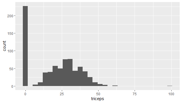
取得できなかったデータを0にしているのでしょう。0をNAに置き換えるデータクリーニングをします。
diabetes_clean <- diabetes_orig %>%
  mutate_at(vars(triceps, glucose, pressure, insulin, mass),
            function(.var) {
              if_else(condition = (.var == 0), # if true (i.e. the entry is 0)
                      true = as.numeric(NA),  # replace the value with NA
                      false = .var # otherwise leave it as it is
              )
            })
これで、データの下準備は完了です。
3.2 学習用/予測用データ
学習用と予測用のデータを準備します。データ全体の75%を学習用に、残りの25%を予測用にします。
set.seed(1234)
diabetes_split <- initial_split(diabetes_clean,
                                prop = 0.75)
diabetes_split
<Training/Validation/Total>
<576/192/768>
diabetes_train <- training(diabetes_split) diabetes_test <- testing(diabetes_split)
後々、チューニングやクロスバリデーションを行うために、それ用の学習用データセットにしておきます。
diabetes_cv <- vfold_cv(diabetes_train)
4.機械学習
4.1 レシピ
データの準備ができたので、機械学習を行っていきます。まずは、レシピの準備と正規化等の準備です。
diabetes_recipe <-
  recipe(diabetes ~ pregnant + glucose + pressure + triceps +
           insulin + mass + pedigree + age,
         data = diabetes_clean) %>%
  step_normalize(all_numeric()) %>%
  step_knnimpute(all_predictors())

diabetes_recipe
Data Recipe

Inputs:

      role #variables
   outcome          1
 predictor          8

Operations:

Centering and scaling for all_numeric
K-nearest neighbor imputation for all_predictors
diabetes_train_preprocessed <- diabetes_recipe %>% prep(diabetes_train) %>% juice() diabetes_train_preprocessed
# A tibble: 576 x 9
   pregnant glucose pressure  triceps insulin   mass pedigree      age diabetes
      <dbl>   <dbl>    <dbl>    <dbl>   <dbl>  <dbl>    <dbl>    <dbl> <fct>
 1   0.626    0.854  -0.0162  0.565    0.382   0.167    0.417  1.44    pos
 2  -0.852   -1.19   -0.510   0.00338 -0.741  -0.828   -0.392 -0.179   neg
 3   1.22     1.99   -0.675   0.434    1.25   -1.30     0.549 -0.0939  pos
 4  -1.15     0.497  -2.65    0.565    0.115   1.52     5.28  -0.00859 pos
 5   0.330   -0.183   0.149  -0.184   -0.637  -0.971   -0.831 -0.265   neg
 6  -0.261   -1.41   -1.83    0.284   -0.557  -0.203   -0.693 -0.606   pos
 7   1.81    -0.216  -0.0821  0.00338 -0.0648  0.409   -1.03  -0.350   neg
 8  -0.556    2.44   -0.181   1.50     3.26   -0.274   -0.957  1.70    pos
 9   0.0349  -0.378   1.63    0.303    0.157   0.736   -0.860 -0.265   neg
10   1.81     0.562   0.643   0.153    0.118  -0.757    2.80   2.04    neg
# ... with 566 more rows
4.2 モデル
続いてモデルを定義します。サポートベクトルマシン(SVM)を使ってみます。SVMは、Support Vector Machineの略で教師あり学習に分類され、現在の多くの学習モデルの中では最も優れた識別能力があるとされています。
svm_model <-
  svm_poly() %>%
  set_engine("kernlab") %>%
  set_mode("classification")

svm_model
Polynomial Support Vector Machine Specification (classification)

Computational engine: kernlab
4.3 ワークフロー
これらをまとめてworkflowにします。ここでは、workflowのフレームワークを作っただけで予測モデル化やチューニングは行っていません。
svm_workflow <- workflow() %>%
  add_recipe(diabetes_recipe) %>%
  add_model(svm_model)

svm_workflow
== Workflow ====================================================================
Preprocessor: Recipe
Model: svm_poly()

-- Preprocessor ----------------------------------------------------------------
2 Recipe Steps

* step_normalize()
* step_knnimpute()

-- Model -----------------------------------------------------------------------
Polynomial Support Vector Machine Specification (classification)

Computational engine: kernlab
4.4 パラメータチューニング
mtryにてチューニング用パラメータを準備したので、どのパラメータが最適かを予測前に確かめます。
svm_grid <- expand.grid(mtry = c(3, 4, 5))
svm_tune_results <- svm_workflow %>%
  tune_grid(resamples = diabetes_cv,
            grid = svm_grid,
            metrics = metric_set(accuracy, roc_auc)
svm_tune_results %>%
  collect_metrics()
# A tibble: 2 x 5
  .metric  .estimator  mean     n std_err
  <chr>    <chr>      <dbl> <int>   <dbl>
1 accuracy binary     0.781    10  0.0199
2 roc_auc  binary     0.839    10  0.0176
さて、この結果は良いのでしょうか?8割ぐらい当たっていればOKでしょうか?
param_final <- svm_tune_results %>%
  select_best(metric = "accuracy")
param_final

svm_workflow <- svm_workflow %>%
  finalize_workflow(param_final)

svm_workflow <- svm_workflow %>%
  finalize_workflow(param_final)
4.5 テスト用データで評価
テスト用データでモデルの評価を行います。
svm_fit <- svm_workflow %>%
  # fit on the training set and evaluate on test set
  last_fit(diabetes_split)

svm_fit
# Monte Carlo cross-validation (0.75/0.25) with 1 resamples
# A tibble: 1 x 6
  splits        id           .metrics      .notes        .predictions    .workflow
  <list>        <chr>        <list>        <list>        <list>          <list>
1 <split [576/~ train/test ~ <tibble [2 x~ <tibble [0 x~ <tibble [192 x~ <workflo~
test_performance <- svm_fit %>% collect_metrics() test_performance
# A tibble: 2 x 3
  .metric  .estimator .estimate
  <chr>    <chr>          <dbl>
1 accuracy binary         0.719
2 roc_auc  binary         0.811
テストでの予測値を見てみます。
test_predictions <- svm_fit %>% collect_predictions()
test_predictions
# A tibble: 192 x 6
   id               .pred_neg .pred_pos  .row .pred_class diabetes
   <chr>                <dbl>     <dbl> <int> <fct>       <fct>
 1 train/test split     0.946    0.0538     4 neg         neg
 2 train/test split     0.546    0.454     10 neg         pos
 3 train/test split     0.109    0.891     12 pos         pos
 4 train/test split     0.680    0.320     19 neg         neg
 5 train/test split     0.752    0.248     22 neg         neg
 6 train/test split     0.717    0.283     30 neg         neg
 7 train/test split     0.861    0.139     39 neg         pos
 8 train/test split     0.605    0.395     40 neg         pos
 9 train/test split     0.183    0.817     41 pos         neg
10 train/test split     0.890    0.110     43 neg         neg
# ... with 182 more rows
confusion matrixで結果を見てみます。
test_predictions %>%
  conf_mat(truth = diabetes, estimate = .pred_class)
Truth
Prediction neg pos
neg 110 38
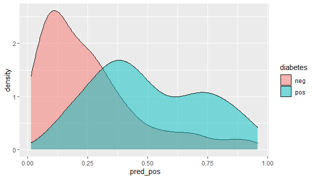
pos 16 28予測された確率分布をグラフで見てみます。
test_predictions %>%
  ggplot() +
  geom_density(aes(x = .pred_pos, fill = diabetes),
               alpha = 0.5)
4.6 モデルの決定
以上の結果から、モデルを決定します。これで、新しいデータに対してモデルを使って予測できるようになります。
final_model <- fit(svm_workflow, diabetes_clean)
final_model
== Workflow [trained] ==========================================================
Preprocessor: Recipe
Model: svm_poly()

-- Preprocessor ----------------------------------------------------------------
2 Recipe Steps

* step_normalize()
* step_knnimpute()

-- Model -----------------------------------------------------------------------
Support Vector Machine object of class "ksvm"

SV type: C-svc  (classification)
 parameter : cost C = 1

Polynomial kernel function.
 Hyperparameters : degree =  1  scale =  1  offset =  1

Number of Support Vectors : 397

Objective Function Value : -391.3924
Training error : 0.230469
Probability model included.
4.7 モデルを使った予測
新しいデータを準備して予測してみます。ある女性のデータを下記のように決めます。
new_woman <- tribble(~pregnant, ~glucose, ~pressure, ~triceps, ~insulin, ~mass, ~pedigree, ~age,
                     2, 95, 70, 31, 102, 28.2, 0.67, 47)
new_woman
# A tibble: 1 x 8
  pregnant glucose pressure triceps insulin  mass pedigree   age
     <dbl>   <dbl>    <dbl>   <dbl>   <dbl> <dbl>    <dbl> <dbl>
1        2      95       70      31     102  28.2     0.67    47
予測してみます。
predict(final_model, new_data = new_woman)
# A tibble: 1 x 1
  .pred_class
  <fct>
1 neg
ということで、糖尿病ではありませんでした。
5.おわりに
Tidymodelsを使って機械学習をする一連の流れを見ました。自分でも、それなりに理解してきた感じです。これからも、もっともっと例題をこなしていきたいです。
