【Python】Kerasを使ってみる（fashion-MNIST）

こちらのページは、RにてKerasを使いましたが、今度はPythonで使ってみます。Pythonでkerasを使うにあたり、こちらのページを参考にさせていただきました。

データをトレーニング用とテスト用に分けて読み込みます。

import keras
import matplotlib.pyplot as plt

(x_train, y_train), (x_test, y_test) = keras.datasets.fashion_mnist.load_data()

データの形を確認してみます。

x_train.shape

(10000, 28, 28)

x_test.shape

(10000, 28, 28)

トレーニング用データの最初の25個を画像として表示してみます（実際の画像は省略）。

plt.figure(figsize=(12,15))
for i in range(25):
    plt.subplot(5, 5, i+1)
    plt.title("Label: " + str(i))
    plt.imshow(x_train[i].reshape(28,28), cmap=None)

トレーニング用データの正解ラベルを表示してみます。

y_train[0:25]

array([9, 0, 0, 3, 0, 2, 7, 2, 5, 5, 0, 9, 5, 5, 7, 9, 1, 0, 6, 4, 3, 1,
       4, 8, 4], dtype=uint8)

x_train = x_train.reshape((60000, 28 * 28))
x_train = x_train.astype('float32') / 255
 
x_test = x_test.reshape((10000, 28 * 28))
x_test = x_test.astype('float32') / 255

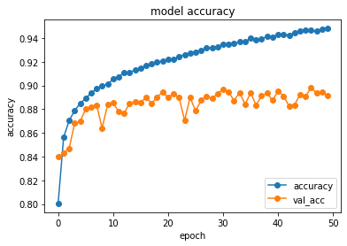
def plot_history(history):

    plt.plot(history.history['accuracy'],"o-",label="accuracy")
    plt.plot(history.history['val_accuracy'],"o-",label="val_acc")
    plt.title('model accuracy')
    plt.xlabel('epoch')
    plt.ylabel('accuracy')
    plt.legend(loc="lower right")
    plt.show()
 

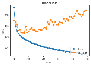
    plt.plot(history.history['loss'],"o-",label="loss",)
    plt.plot(history.history['val_loss'],"o-",label="val_loss")
    plt.title('model loss')
    plt.xlabel('epoch')
    plt.ylabel('loss')
    plt.legend(loc='lower right')
    plt.show()

モデルを作ります。

from keras.models import Sequential
from keras.layers import Activation, Dense, Dropout
from keras.optimizers import RMSprop
 
model = keras.models.Sequential()
model.add(Dense(units=512,input_dim=28*28))
model.add(Activation('relu'))
model.add(Dropout(0.2))
model.add(Dense(units=10))
model.add(Activation('softmax'))
model.compile(loss='sparse_categorical_crossentropy',optimizer=RMSprop(),metrics=['accuracy'])

学習します。

history = model.fit(x_train, y_train,
                    batch_size=128,
                    epochs=50,
                    verbose=1,
                    validation_data=(x_test, y_test))

Epoch 1/50
469/469 [==============================] - 4s 3ms/step - loss: 0.7545 - accuracy: 0.7407 - val_loss: 0.4480 - val_accuracy: 0.8396
Epoch 2/50
469/469 [==============================] - 1s 3ms/step - loss: 0.4050 - accuracy: 0.8520 - val_loss: 0.4363 - val_accuracy: 0.8430
Epoch 3/50
469/469 [==============================] - 1s 3ms/step - loss: 0.3579 - accuracy: 0.8678 - val_loss: 0.4078 - val_accuracy: 0.8467
Epoch 4/50
469/469 [==============================] - 1s 3ms/step - loss: 0.3329 - accuracy: 0.8759 - val_loss: 0.3575 - val_accuracy: 0.8681
Epoch 5/50
469/469 [==============================] - 1s 3ms/step - loss: 0.3164 - accuracy: 0.8823 - val_loss: 0.3645 - val_accuracy: 0.8695
Epoch 6/50
469/469 [==============================] - 1s 3ms/step - loss: 0.3039 - accuracy: 0.8876 - val_loss: 0.3392 - val_accuracy: 0.8800
Epoch 7/50
469/469 [==============================] - 1s 3ms/step - loss: 0.2876 - accuracy: 0.8953 - val_loss: 0.3371 - val_accuracy: 0.8817
Epoch 8/50
・・・・・・・・・・・・・・・・・

plot_history(history)

score = model.evaluate(x_test, y_test, verbose=1)
 
print('loss=', score[0])
print('accuracy=', score[1])

313/313 [==============================] - 1s 2ms/step - loss: 0.5373 - accuracy: 0.8915
loss= 0.5373466610908508
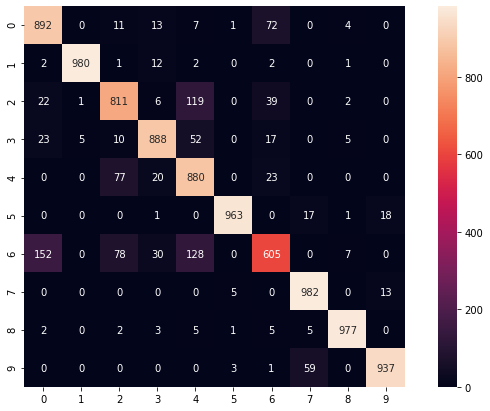
accuracy= 0.8914999961853027

import numpy as np
from sklearn.metrics import confusion_matrix

predict_classes = model.predict_classes(x_test)
true_classes = y_test
print(confusion_matrix(true_classes, predict_classes))

/usr/local/lib/python3.6/dist-packages/tensorflow/python/keras/engine/sequential.py:450: UserWarning: `model.predict_classes()` is deprecated and will be removed after 2021-01-01. Please use instead:* `np.argmax(model.predict(x), axis=-1)`,   if your model does multi-class classification   (e.g. if it uses a `softmax` last-layer activation).* `(model.predict(x) > 0.5).astype("int32")`,   if your model does binary classification   (e.g. if it uses a `sigmoid` last-layer activation).
  warnings.warn('`model.predict_classes()` is deprecated and '

[[892   0  11  13   7   1  72   0   4   0]
 [  2 980   1  12   2   0   2   0   1   0]
 [ 22   1 811   6 119   0  39   0   2   0]
 [ 23   5  10 888  52   0  17   0   5   0]
 [  0   0  77  20 880   0  23   0   0   0]
 [  0   0   0   1   0 963   0  17   1  18]
 [152   0  78  30 128   0 605   0   7   0]
 [  0   0   0   0   0   5   0 982   0  13]
 [  2   0   2   3   5   1   5   5 977   0]
 [  0   0   0   0   0   3   1  59   0 937]]

import pandas as pd
import seaborn as sn
from sklearn.metrics import confusion_matrix
import matplotlib.pyplot as plt
 
def print_cmx(y_true, y_pred):
    labels = sorted(list(set(y_true)))
    cmx_data = confusion_matrix(y_true, y_pred, labels=labels)
    
    df_cmx = pd.DataFrame(cmx_data, index=labels, columns=labels)
 
    plt.figure(figsize = (12,7))
    sn.heatmap(df_cmx, annot=True, fmt='g' ,square = True)
    plt.show()
 
print_cmx(true_classes, predict_classes)