【R】feasts

1. はじめに

feastsは、時系列データを扱いやすくしてくれるパッケージです。

2. インストール

CRANからインストールできます。

install.packages("feasts")

3. 使ってみる

オーストラリアのたばこ消費量の四半期ごとのデータを年別で表示してみます。

library(feasts)
library(tsibble)
library(tsibbledata)
library(tidyverse)
library(ggplot2)
library(lubridate)

aus_production %>% gg_season(Tobacco)

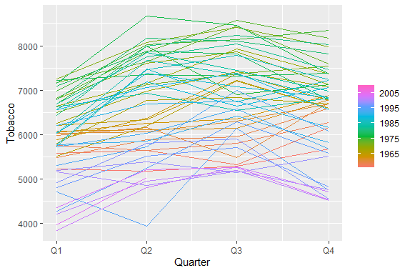
季節の変動に規則性はないようですが、年を追うごとに消費量は減っているようですね。

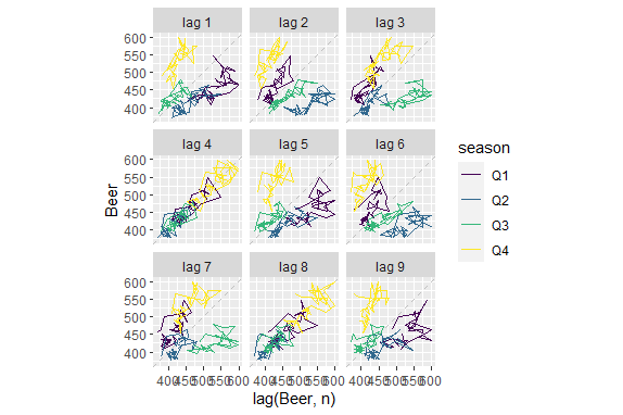
aus_production %>% filter(year(Quarter) > 1970) %>% gg_lag(Beer)

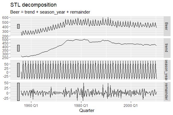
dcmp <- aus_production %>%
  model(STL(Beer ~ season(window = Inf)))
components(dcmp)

> components(dcmp)
# A dable:           218 x 7 [1Q]
# Key:               .model [1]
# STL Decomposition: Beer = trend + season_year + remainder
   .model Quarter  Beer trend season_year remainder season_adjust
   <chr>    <qtr> <dbl> <dbl>       <dbl>     <dbl>         <dbl>
 1 STL(B~ 1956 Q1   284  272.        2.14     10.1           282.
 2 STL(B~ 1956 Q2   213  264.      -42.6      -8.56          256.
 3 STL(B~ 1956 Q3   227  258.      -28.5      -2.34          255.
 4 STL(B~ 1956 Q4   308  253.       69.0     -14.4           239.
 5 STL(B~ 1957 Q1   262  257.        2.14      2.55          260.
 6 STL(B~ 1957 Q2   228  261.      -42.6       9.47          271.
 7 STL(B~ 1957 Q3   236  263.      -28.5       1.80          264.
 8 STL(B~ 1957 Q4   320  264.       69.0     -12.7           251.
 9 STL(B~ 1958 Q1   272  266.        2.14      4.32          270.
10 STL(B~ 1958 Q2   233  266.      -42.6       9.72          276.
# ... with 208 more rows

components(dcmp) %>% autoplot()

4. さいごに

なかなか使いやすいパッケージです。